Joint & Marginal
7 minute read
In this section, we will understand Joint, Marginal & Conditional Probability.
So far, we have dealt with a single random variable.
Now, let’s explore the probability distributions of 2 or more random variables occurring together.
Joint Probability Distribution:
It describes the probability of 2 or more random variables occurring simultaneously.
- The random variables can be from different distributions, such as, discrete and continuous.
Joint CDF:
Discrete Case:
Continuous Case:
Joint PMF:
Key Properties:
- \(P(X = x, Y = y) \ge 0 ~ \forall (x,y) \)
- \( \sum_{i} \sum_{j} P(X = x_i, Y = y_j) = 1 \)
Joint PDF:
Key Properties:
- \(f_{X,Y}(x,y) \ge 0 ~ \forall (x,y) \)
- \( \int_{-\infty}^{\infty} \int_{-\infty}^{\infty} f_{X,Y}(x,y) dy dx = 1 \)
- If we consider 2 random variables, say, height(X) and weight(Y), then the joint distribution will tell us
the probability of finding a person having a particular height and weight.
A ball is picked at random from each bag, such that both draws are independent of each other.
Let’s use this example to understand joint probability.
Let A & B be discrete random variables associated with the outcome of the ball drawn from first and second bags
respectively.
| A = Red | A = Blue | |
|---|---|---|
| B = Red | 2/5*3/5 = 6/25 | 3/5*3/5 = 9/25 |
| B = Blue | 2/5*2/5 = 4/25 | 3/5*2/5 = 6/25 |
Since, the draws are independent, joint probability = P(A) * P(B)
Each of the 4 cells in above table shows the probability of combination of results from 2 draws or joint probability.
Marginal Probability Distribution:
It describes the probability distribution of an individual random variable in a joint distribution,
without considering the outcomes of other random variables.
- If we have the joint distribution, then we can get the marginal distribution of each random variable from it.
- Marginal probability equals summing the joint probability across other random variables.
Marginal CDF:
We know that Joint CDF =
Marginal CDF =
\[ F_X(a, \infty) = P(X \le a, Y < \infty) = P(X \le a) \]Discrete Case:
Continuous Case:
Law of Total Probability
We know that Joint Probability Distribution =
The events \((Y=y)\) partition the sample space, such that:
- \( (Y=y_1) \cap (Y=y_2) \cap ... \cap (Y=y_n) = \Phi \)
- \( (Y=y_1) \cup (Y=y_2) \cup ... \cup (Y=y_n) = \Omega \)
From Law of Total Probability, we get:
Marginal PMF:
Marginal PDF:
X: Roll a die ; \( \Omega = \{1,2,3,4,5,6\} \)
Y: Toss a coin ; \( \Omega = \{H,T\} \)
Joint PMF = \( P_{X,Y}(x,y) = P(X=x, Y=y) = 1/6*1/2 = 1/12\)
Marginal PMF of X = \( P_X(x) =\sum_{y \in \mathbb{\{H,T\}}} P_{X,Y}(x,y) = = 1/12+1/12 = 1/6\)
=> Marginally, X is uniform over 1-6 i.e a fair die.
Marginal PMF of Y = \( P_Y(y) = \sum_{1}^6 P_{X,Y}(x,y) = 6*(1/12) = 1/2 \)
=> Marginally, Y is uniform over H,T i.e a fair coin.
\( X \sim U(0,1) \)
\( Y \sim U(0,1) \)
Marginal PDF = \(f_X(x) = \int_{-\infty}^{\infty} f_{X,Y}(x,y) dy \)
Joint PDF =
Marginal PDF =
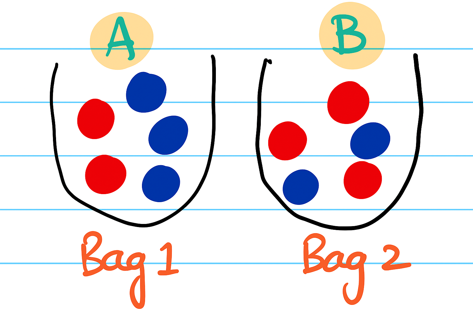
\[ \begin{aligned} f_X(x) &= \int_{0}^{1} f_{X,Y}(x,y) dy \\ &= \int_{0}^{1} 1 dy \\ &= 1 \\ f_X(x) &= \begin{cases} 1 & \text{if } x \in [0,1] \\ 0 & \text{otherwise } \end{cases} \end{aligned} \]There are 2 bags; bag_1 has 2 red balls & 3 blue balls, bag_2 has 3 red balls & 2 blue balls.
A ball is picked at random from each bag, such that both draws are independent of each other.
Let’s use this example to understand marginal probability.
Let A & B be discrete random variables associated with the outcome of the ball drawn from first and second bags
respectively.
| A = Red | A = Blue | P(B) (Marginal) | |
|---|---|---|---|
| B = Red | 2/5*3/5 = 6/25 | 3/5*3/5 = 9/25 | 6/25 + 9/25 = 15/25 = 3/5 |
| B = Blue | 2/5*2/5 = 4/25 | 3/5*2/5 = 6/25 | 4/25 + 6/25 = 10/25 = 2/5 |
| P(A) (Marginal) | 6/25 + 4/25 = 10/25 = 2/5 | 9/25 + 6/25 = 15/25 = 3/5 |
We can see from the table above - P(A=Red) is the sum of joint distribution over all possible values of B i.e Red & Blue.
Conditional Probability:
It measures the probability of an event occurring given that another event has already happened.
- It provides a way to update our belief about the likelihood based on new information.
P(A, B) = Joint Probability of A and B
P(B) = Marginal Probability of B
=> Conditional Probability = Joint Probability / Marginal Probability
Conditional CDF:
Discrete Case:
Continuous Case:
Conditional PMF:
Conditional PDF:
Application:
- Generative machine learning models, such as, GANs, learn the conditional distribution of pixels, given the style of input image.
Note: We only have information about the joint and marginal probabilities.
What is the conditional probability of drawing a red ball in the first draw, given that a blue ball is drawn in second draw?
Let A & B be discrete random variables associated with the outcome of the ball drawn from first and second bags
respectively.
A = Red ball in first draw
B = Blue ball in second draw.
| A = Red | A = Blue | P(B) (Marginal) | |
|---|---|---|---|
| B = Red | 6/25 | 9/25 | 3/5 |
| B = Blue | 4/25 | 6/25 | 2/5 |
| P(A) (Marginal) | 2/5 | 3/5 |
Therefore, probability of drawing a red ball in the first draw, given that a blue ball is drawn in second draw = 2/5.
Conditional Expectation:
This gives us the conditional expectation of a random variable X, given another random variable Y=y.
Discrete Case:
Continuous Case:
For example:
- Conditional expectation of of a person’s weight, given his/her height = 165 cm, will give us the average weight of all people with height = 165 cm.
Applications:
- Linear regression algorithm is conditional expectation of target variable ‘Y’, given input feature variable ‘X’.
- Expectation Maximisation(EM) algorithm is built on conditional expectation.
Conditional Variance:
This gives us the variance of a random variable calculated after taking into account the value(s) of another related variable.
For example:
- Variance of car’s mileage for city driving might be small, but the variance will be large for mix of city and highway driving.
Note: Models that take into account the change in variance or heteroscedasticity tend to be more accurate.
End of Section