Parametric Model Estimation
16 minute read
In this section, we will understand Parametric Model Estimation via two philosophical approaches.
- Frequentist: Parameter \(\Theta\) is fixed, but unknown.
- Bayesian: Parameter \(\Theta\) itself is unknown, so we model it as a random variable with a probability distribution.
Parametric Model Estimation:
It is the process of finding the best-fitting finite set of parameters \(\Theta\) for a model that assumes a
specific probability distribution for the data.
It involves using the dataset to estimate the parameters (like the mean and standard deviation of a normal distribution)
that define the model.
\(P(X \mid \Theta) \) : Probability of seeing data \(X: (X_1, X_2, \dots, X_n) \), given the parameters \(\Theta\) of the
underlying probability distribution from which the data is assumed to be generated.
Goal of estimation:
We observed data, \( D = \{X_1, X_2, \dots, X_n\} \), and we want to infer the the unknow parameters \(\Theta\)
of the underlying probability distribution, assuming that the data is generated I.I.D.
Read more for I.I.D
Note: Most of the time, from experience, we know the underlying probability distribution of data, such as, Bernoulli, Gaussian, etc.
There are 2 philosophical approaches to estimate the parameters of a parametric model:
- Frequentist:
- Parameters \(\Theta\) is fixed, but unknown, only data is random.
- It views probability as the long-run frequency of events in repeated trials; e.g toss a coin ’n’ times.
- It is favoured when the sample size is large.
- For example, Maximum Likelihood Estimation(MLE), Method of Moments, etc.
- Bayesian:
- Parameters \(\Theta\) itself is unknown, so we model it as a random variable with a probability distribution.
- It views probability as a degree of belief that can be updated with new evidence, i.e. data.
Thus, integrating prior knowledge with data to express the uncertainty about the parameters. - It is favoured when the sample size is small, as it uses prior belief about the data distribution too.
- For example, Maximum A Posteriori Estimation(MAP), Minimum Mean Square Error Estimation(MMSE), etc..
Maximum Likelihood Estimation:
It is the most popular frequentist approach to estimate the parameters of a model.
This method helps us find the parameters \(\Theta\) that make the data most probable.
Likelihood Function:
Say, we have data, \(D = X_1, X_2, \dots, X_n\) are I.I.D discrete random variable with PMF = \(P_{\Theta}(.)\)
Then, the likelihood function is the probability of observing the data, \(D = \{X_1, X_2, \dots, X_n\}\),
given the parameters \(\Theta\).
Task:
Find the value of parameter \(\Theta_{ML}\) that maximizes the likelihood function.
In order to find the parameter \(\Theta_{ML}\) that maximises the likelihood function,
we need to take the first derivative of the likelihood function with respect to \(\Theta\) and equate it to zero.
But, taking derivative of a product is challenging, so we will take the logarithm on both sides.
Note: Log is a monotonically increasing function, i.e, as x increases, log(x) increases too.
Let us denote the log-likelihood function as \(\bar{L}\).
\[ \begin{aligned} \mathcal{\bar{L}_{X_1, X_2, \dots ,X_n}}(\Theta) &= log [\prod_{i=1}^{n} P_{\Theta}(X_i)] \\ &= \sum_{i=1}^{n} log P_{\Theta}(X_i) \\ \end{aligned} \]Therefore, Maximum Likelihood Estimation is the parameter \(\Theta_{ML}\) that maximises the log-likelihood function.
\[ \Theta_{ML}(X_1, X_2, \dots, X_n) = \underset{\Theta}{\mathrm{argmax}}\ \bar{L}_{X_1, X_2, \dots ,X_n}(\Theta) \]Given \(X_1, X_2, \dots, X_n\) are I.I.D. Bernoulli random variable with PMF as below:
Estimate the parameter \(\theta\) using Maximum Likelihood Estimation.
Let, \(n_1 = \) number of 1’s in the dataset.
Likelihood Function:
Log-Likelihood Function:
Maximum Likelihood Estimation:
In order to find the parameter \(\theta_{ML}\), we need to take the first derivative of the log-likelihood function
with respect to \(\theta\) and equate it to zero.
Say, e.g., we have 10 observations for the Bernoulli random variable as: 1,0,1,1,0,1,1,0,1,0.
Then, the parameter \(\Theta_{ML} = \frac{6}{10} = 0.6\) i.e proportion of 1’s.
\(x_1, x_2, \dots, x_n\) are the realisations/observations of the random variable.
Estimate the parameters \(\mu\) and \(\sigma\) of the Gaussian distribution using Maximum Likelihood Estimation.
Likelihood Function:
Log-Likelihood Function:
Note: Here, the first term \( -\frac{n}{2} log (2\pi) \) is a constant wrt both \(\mu\) and \(\sigma\), so we can ignore the term.
Maximum Likelihood Estimation:
Instead of finding \(\mu\) and \(\sigma\) that maximises the log-likelihood function,
we can find \(\mu\) and \(\sigma\) that minimises the negative of the log-likelihood function.
Now, lets differentiate the log likelihood function wrt \(\mu\) and \(\sigma\) separately to get \(\mu_{ML}, \sigma_{ML}\).
Lets, calculate \(\mu_{ML}\) first by taking the derivative of the log-likelihood function wrt \(\mu\) and equating it to 0.
Similarly, we can calculate \(\sigma_{ML}\) by taking the derivative of the log-likelihood function wrt \(\sigma\)
and equating it to 0.
Note: In general MLE is biased, i.e does NOT give an unbiased estimate => divides by \(n\) instead of \((n-1)\).
Bayesian Statistics:
Bayesian statistics model parameters by updating initial beliefs (prior probabilities) with observed data to form
a final belief (posterior probability) using Bayes’ Theorem.
Instead of a single point estimate, it provides a probability distribution over possible parameter values,
which allows to quantify uncertainty and yields more robust models, especially with limited data.
Bayes’ Theorem:
\(P(\Theta)\): Prior: Initial distribution of \(\Theta\) before seeing the data.
\(P(X \mid \Theta)\): Likelihood: Conditional distribution of data \(X\), given the parameter \(\Theta\).
\(P(\Theta \mid X)\): Posterior: Conditional distribution of parameter \(\Theta\), given the data \(X\).
\(P(X)\): Evidence: Probability of seeing the data \(X\).
\(x_1, x_2, \dots, x_n\) are the realisations, \(\Theta \in [0, 1] \).
Estimate the parameter \(\Theta\) using Bayesian statistics.
Let, \(n_1 = \) number of 1’s in the dataset.
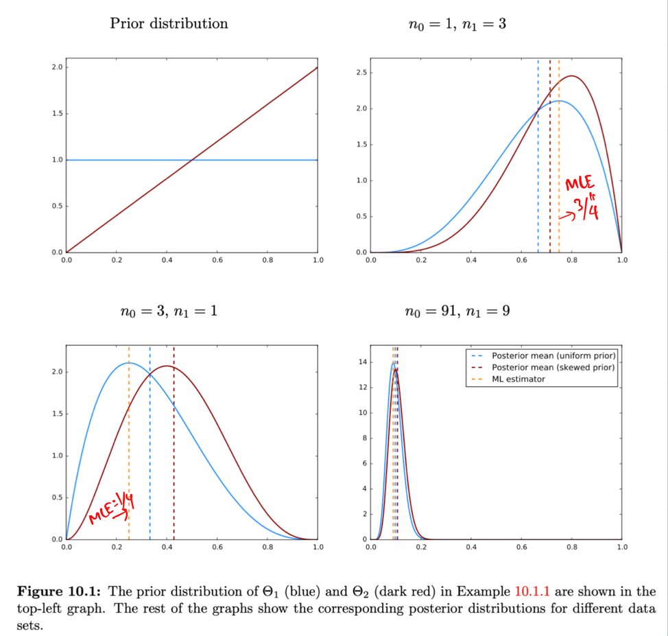
Prior: \(P(\Theta)\) : \(\Theta \sim U(0, 1) \), i.e, parameter \(\Theta\) comes from a continuos uniform
distribution in the range [0,1].
\(f_{\Theta}(\theta) = 1, \theta \in [0, 1] \)
Likelihood: \(P_{X \mid \Theta}(x \mid \theta) = \theta^{n_1} (1 - \theta)^{n - n_1} \).
Posterior:
\[ f_{\Theta \mid X} (\theta \mid x) = \frac{f_{\Theta}(\theta) P_{X \mid \Theta}(x \mid \theta)}{f_{X}(x)} \\ \]Note: The most difficult part is to calculate the denominator \(f_{X}(x)\).
So, either we try NOT to compute it all together, or we try to map it to some known functions to make calculations easier.
We know that we can get the marginal probability by integrating the joint probability over another variable.
Also from conditional probability, we know:
\[ \tag{2} f_{X \mid Y}(x \mid y) = \frac{f_{X,Y}(x,y)}{f_{Y}(y)} \\ => f_{X,Y}(x,y) = f_{Y}(y) f_{X \mid Y}(x \mid y) \]From equations 1 and 2, we have:
\[ \tag{3} f_{X}(x) = \int_{Y}f_{Y}(y) f_{X \mid Y}(x \mid y)dy \]Now let’s replace the value of \(f_{X}(x) \) in the posterior from equation 3:
Posterior:
Beta Function:
It is a special mathematical function denoted by B(a, b) or β(a, b) that is defined by the integral formula:
Note: We can see that the denominator of the posterior is of the form of Beta function.
Posterior:
Suppose, in the above example, we are told that the parameter \(\Theta\) is closer to 1 than 0.
How will we incorporate this useful information (apriori knowledge) into our parameter estimation?
Since, we know apriori that \(\Theta\) is closer to 1 than 0, we should take this initial belief into account
to do our parameter estimation.
Prior:
Posterior:
\[ \begin{aligned} f_{\Theta \mid X} (\theta \mid x) &= \frac{f_{\Theta}(\theta) P_{X \mid \Theta}(x \mid \theta)}{f_{X}(x)} \\[10pt] &= \frac{f_{\Theta}(\theta) P_{X \mid \Theta}(x \mid \theta)}{\int_{\Theta}f_{\Theta}(\theta) P_{X \mid \Theta}(x \mid \theta)d\theta} \\[10pt] &= \frac{f_{\Theta}(\theta) P_{X \mid \Theta}(x \mid \theta)}{\int_{0}^1f_{\Theta}(\theta) P_{X \mid \Theta}(x \mid \theta)d\theta} \\[10pt] \text{ We know that: } f_{\Theta}(\theta) = 2\Theta, \theta \in [0, 1] \\ &= \frac{2\Theta * P_{X \mid \Theta}(x \mid \theta)}{\int_{0}^1 2\Theta* P_{X \mid \Theta}(x \mid \theta)d\theta} \\[10pt] & = \frac{2\Theta * \theta^{n_1} (1 - \theta)^{n - n_1}}{\int_{0}^1 2\Theta * \theta^{n_1} (1 - \theta)^{n - n_1}} \\[10pt] => f_{\Theta \mid X} (\theta \mid x) &= \frac{\theta^{n_1+1} (1 - \theta)^{n - n_1}}{β(n_1+2, n-n_1+1)} \end{aligned} \]Note: If we do NOT have enough data, then we should NOT ignore our intial belief.
However, if we have enough data, then the data will override our initial belief and the posterior will be dominated by data.
Note: Bayesian approach gives us a probability distribution of parameter \(Theta\).
We can use Bayesian Point Estimators, after getting the posterior distribution, to summarize it with a single value for
practical use, such as,
- Maximum A Posteriori (MAP) Estimator
- Minimum Mean Square Error (MMSE) Estimator
Maximum A Posteriori (MAP) Estimator:
It finds the mode(peak) of the posterior distribution.
- MAP has the minimum probability of error, since it picks single most probable value.
Estimate the unknown parameter \(\mu\) using MAP.
Given that :
\(\Theta\) is discrete, with probability 0.5 for both 0 and 1.
=> The Gaussian distribution is equally likely to be centered at 0 or 1.
Variance: \(\sigma^2 = 1\)
Prior:
Likelihood:
Posterior:
We need to find:
\[ \underset{\Theta}{\mathrm{argmax}}\ P_{\Theta \mid X} (\theta \mid x) \]Taking log on both sides:
Let’s calculate the log-likelihood function first -
\[ \begin{aligned} \log f_{X \mid \Theta}(x \mid \theta) &= \log \prod_{i=1}^n \frac{1}{\sqrt{2\pi}} e^{-\frac{(x_i-\theta)^2}{2}} \\ &= log(\frac{1}{\sqrt{2\pi}})^n + \sum_{i=1}^n \log (e^{-\frac{(x_i-\theta)^2}{2}}), \text{ since \(\sigma = 1\)} \\ &= n\log(\frac{1}{\sqrt{2\pi}}) + \sum_{i=1}^n -\frac{(x_i-\theta)^2}{2} \\ => \tag{2} \log f_{X \mid \Theta}(x \mid \theta) &= n\log(\frac{1}{\sqrt{2\pi}}) - \sum_{i=1}^n \frac{(x_i-\theta)^2}{2} \end{aligned} \]Here computing \(f_{X}(x)\) is difficult.
So, instead of differentiating above equation wrt \(\Theta\), and equating to 0,
we will calculate the above expression for \(\theta=0\) and \(\theta=1\) and compare the values.
This way we can get rid of the common value \(f_{X}(x)\) in both expressions that is not dependent on \(\Theta\).
When \(\theta=1\):
Similarly, when \(\theta=0\):
So, we can say that \(\theta = 1\) only if :
the value of the above expression for \(\theta = 1\) > the value of the above expression for \(\theta = 0\)
From equation 3 and 4:
Note: If the prior is uniform then \(\Theta_{MAP} = \Theta_{MLE}\), because uniform prior does NOT give any information about the initial bias, and all possibilities are equally likely.
What if, in the above example, we know that the initial belief is not uniform but biased towards 0?
Prior:
Now, let’s compare the log-posterior for both the cases i.e \(\theta=0\) and \(\theta=1\) as we did earlier.
But, note that this time the probabilities for \(\theta=0\) and \(\theta=1\) are different.
So, we can say that \(\theta = 1\) only if :
the value of the above expression for \(\theta = 1\) > the value of the above expression for \(\theta = 0\)
From equation 3 and 4 above:
Therefore, we can see that \(\Theta_{MAP}\) is extra biased towards 0.
Note: For a non-uniform prior \(\Theta_{MAP}\) estimate will be pulled towards the prior’s mode.
e.g: Patient has a certain disease or not.
But, what if we want to minimize average magnitude of errors, over time, say predicting a stock’s price?
Just getting to know whether the prediction was right or wrong is not sufficient here.
We also want to know that the prediction was wrong by how much, so that we can minimize the loss over time.
Minimum Mean Square Error (MMSE) Estimation:
Minimizes the expected value of squared error.
Mean of the posterior distribution is the conditional expectation of parameter \(\Theta\), given the data.
- Posterior mean minimizes the the mean squared error.
\(\hat\Theta(X)\): Predicted value.
\(\Theta\): Actual value.
Let’s revisit the above examples that we used for MLE.
Case 1: Uniform Continuous Prior for parameter \(\Theta\) of Bernoulli distribution
Prior:
Posterior:
Let’s calculate the \(\Theta_{MMSE}\):
Similarly, for the second case where the prior is biased towards 1.
Case 2: Prior is biased towards 1 for parameter \(\Theta\) of Bernoulli distribution
Prior:
Posterior:
So, here in this case our \(\Theta_{MMSE}\) is:
MAP vs MMSE
- MMSE is the average of the posterior distribution, whereas MAP is the mode/peak.
- If posterior distribution is symmetric and unimodal(only 1 peak), then MAP and MMSE are very close.
- If posterior distribution is skewed and multimodal(many peaks), then MAP and MMSE can differ a lot.
- MMSE considers all the values of the posterior distribution, hence it is more accurate than MAP, especially for skewed or multimodal distributions.
End of Section