Probability Density Function
9 minute read
This is a function used for continuous random variables to describe the likelihood of the variable taking on a value
within a specific range or interval.
Since, at any given point the probability of a continuous random variable is zero,
we find the probability within a given range.
Note: Called ‘density’ because probability is spread continuously over a range of values
rather than being concentrated at a single point as in PMF.
e.g: Uniform, Gaussian, Exponential, etc.
Note: PDF is a continuous function \(f(x)\).
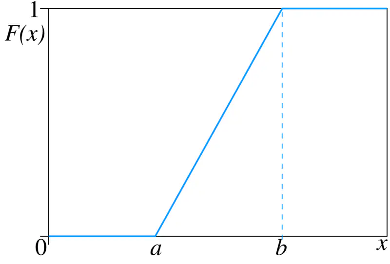
It is also the derivative of Cumulative Distribution Function (CDF) \(F_X(x)\)
\(PDF = f(x) = F'(X) = \frac{dF_X(x)}{dx} \)
- Non-Negative: Function must be non-negative everywhere i.e \(f(x) \ge 0 \forall x\).
- Sum = 1: Total area under curve must be equal to 1.
\( \int_{-\infty}^{\infty} f(x) \,dx = 1\) - Probability of a continuous random variable in the range [a,b] is given by -
\( P(a \le x \le b) = \int_{a}^{b} f(x) \,dx\)
Consider a line segment/interval from \(\Omega = [0,2] \)
Random variable \(X(\omega) = \omega\)
i.e \(X(1) = 1 ~and~ X(1.1) = 1.1 \)
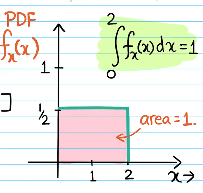
Note: If we know the PDF of a continuous random variable, then we can find the probability of any given region/interval by calculating the area under the curve.
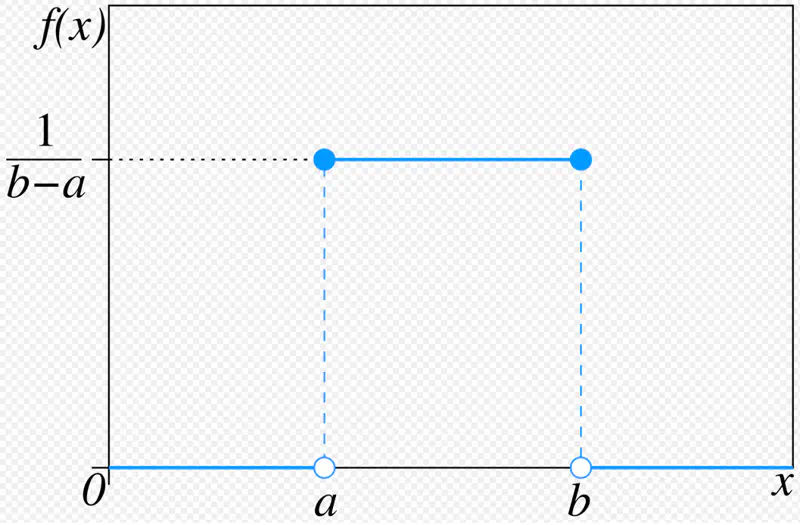
All the outcomes within the given range are equally likely to occur.
Also known as ‘fair’ distribution.
Note: This is a natural starting point to understand randomness in general.
Mean = Median = \( \frac{a+b}{2} ~if~ x \in [a,b] \)
Variance = \( \frac{(b-a)^2}{12} \)
Standard uniform distribution: \( X \sim U(0,1) \)
PDF in terms of mean(\(\mu\)) and standard deviation(\(\sigma\)) -
Random number generator that generates a random number between 0 and 1.
It is a continuous probability distribution characterized by a symmetrical, bell-shaped curve with
most data clustered around the central average, with frequency of values decreasing as they move away from the center.
- Most outcomes are average; extremely low or extremely high values are rare.
- Characterised by mean and standard deviation/variance.
- Peak at mean = median, symmetric around mean.
Note: Most important and widely used distribution.
\[ X \sim N(\mu, \sigma^2) \] $$ \begin{aligned} PDF = f(x) = \dfrac{1}{\sqrt{2\pi}\sigma}e^{-\dfrac{(x-\mu)^2}{2\sigma^2}} \\ \end{aligned} $$
Mean = \(\mu\)
Variance = \(\sigma^2\)
Standard normal distribution:
\[ Z \sim N(0,1) ~i.e~ \mu = 0, \sigma^2 = 1 \]
Any normal distribution can be standardized using Z-score transformation:
- Human height, IQ scores, blood-pressure etc.
- Measurement of errors in scientific experiments.
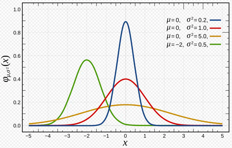
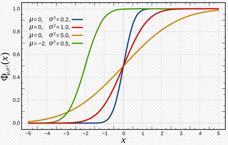
- 68.27% of the data lie within 1 standard deviation of the mean i.e \(\mu \pm \sigma\)
- 95.45% of the data lie within 2 standard deviations of the mean i.e \(\mu \pm 2\sigma\)
- 99.73% of the data lie within 3 standard deviations of the mean i.e \(\mu \pm 3\sigma\)
It is used to model the amount of time until a specific event occurs.
Given that:
- Events occur with a known constant average rate.
- Occurrence of an event is independent of the time since the last event.
Parameters:
Rate parameter: \(\lambda\): Average number of events per unit time
Scale parameter: \(\mu ~or~ \beta \): Mean time between events
Mean = \(\frac{1}{\lambda}\)
Variance = \(\frac{1}{\lambda^2}\)
\[ \lambda = \dfrac{1}{\beta} = \dfrac{1}{\mu}\]
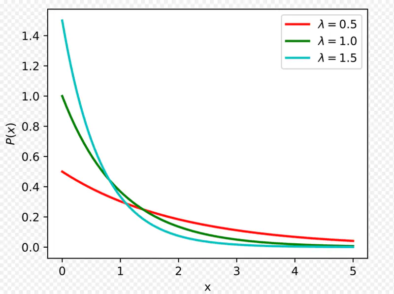
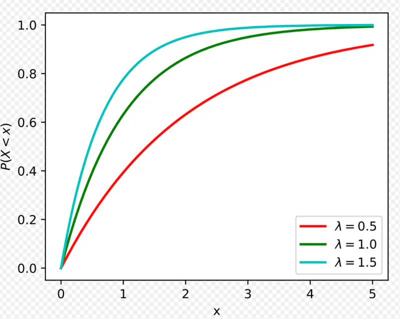
Mean time to serve 1 customer = \(\mu\) = 4 minutes
So, \(\lambda\) = average number of customers served per unit time = \(1/\mu\) = 1/4 = 0.25 minutes
Probability to serve a customer in less than 3 minutes can be found using CDF -
So, probability of a customer being served in less than 3 minutes is 53%(approx).
In this case x = 2 minutes, and \(\lambda\) = 0.25 so,
So, probability of a customer being served in greater than 2 minutes is 60%(approx).
Probability of waiting for an additional period of time for an event to occur is independent of
how long you have already waited.
e.g: Lifetime of electronic items follow exponential distribution.
- Probability of a computer part failing in the next 1 hour is the same regardless of whether
it has been working for 1 day or 1 year or 5 years.
Note: Memoryless property makes exponential distribution particularly useful for -
- Modeling systems that do not experience ‘wear and tear’; where failure is due to a constant random rate rather than degradation over time.
- Also, useful for ‘reliability analysis’ of electronic systems where a ‘random failure’ model is more appropriate than
a ‘wear out’ model.
Task: We want to find the probability of the electronic item lasting for \(x > t+s \) days,
given that it has already lasted for \(x>t\) days.
This is a ‘conditional probability’.
Since,
We want to find: \( P(X > t+s \mid X > t) = ~? \)
Hence, probability that the electronic item will survive for an additional time ’s’ days
is independent of the time ’t’ days it has already survived.
Poisson distribution models the number of events occurring in a fixed interval of time,
given a constant average rate \(\lambda \).
Exponential distribution models the time interval between those successive events.
- 2 faces of the same coin.
- \(\lambda_{poisson}\) is identical to rate parameter \(\lambda_{exponential}\).
Note: If the number of events in a given interval follow a Poisson distribution, then the waiting time between those events will necessarily follow an Exponential distribution.
Lets see the proof for the above statement.
Poisson Case:
The probability of observing exactly ‘k’ events in a time interval of length ’t’
with an average rate of \( \lambda \) events per unit time is given by -
The event that waiting time until next event > t, is same as observing ‘0’ events in that interval.
=> We can use the PMF of Poisson distribution with k=0.
Exponential Case:
Now, lets consider exponential distribution that models the waiting time ‘T’ until next event.
The event that waiting time ‘T’ > t, is same as observing ‘0’ events in that interval.
Observation:
Exponential distribution is a direct consequence of Poisson distribution probability of ‘0’ events.
Using Poisson:
Average failure rate, \(\lambda\) = 1/20 = 0.05
Time interval, t = 10 hours
Number of events, k = 0
Average number of events in interval, (\(\lambda t\)) = (1/20) * 10 = 0.5
Probability of having NO failures in the next 10 hours = ?
Using Exponential:
What is the probability that wait time until next failure > 10 hours?
Waiting time, T > t = 10 hours.
Average number of failures per hour, \(\lambda\) = 1/20 per hour
Therefore, we have seen that this problem can be solved using both Poisson and Exponential distribution.
End of Section