Chi-Square Test

7 minute read

In this section, we will understand Chi-Square Test.

Statistics for AI & ML | Full Course Videos

Note: All the hypothesis tests get their name from the underlying distribution of the test statistic.

📘

Chi-Square Distribution (\(\chi^2\)):
A random variable Q is said to follow a chi-square distribution with ’n’ degrees of freedom,i.e \(\chi^2(n)\),
if it is the sum of squares of ’n’ independent random variables that follow a standard normal distribution, i.e, \(N(0,1)\).

\[ Q = \chi^2(n) = \sum_{i=1}^n Z_i^2 \\ \text{ where: } Z_i \sim N(0,1) \\ \text{ n: degrees of freedom } \]

Key Properties:

Non-negative, since sum of squares.
Asymmetric, right skewed.
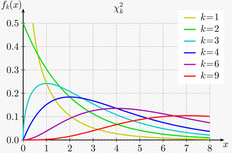
Shape depends on the degrees of freedom; as \(\nu\) increases, the distribution becomes more symmetric and approaches a normal distribution.

Degrees of Freedom (\(\nu\))

It represents the number of independent pieces of information available in the sample to estimate the variability in the data.
Generally speaking, it represents the number of independent values that are free to vary in a dataset when estimating a parameter.
e.g.: If we have k observations and their sum = 50.
The sum of (k-1) terms can be anything, but the kth term is fixed at 50 - (sum of other (k-1) terms).
So, we have only (k-1) terms that can change independently, therefore, the DOF(\(\nu\)) = k-1.

Watch Video

Central Limit Theorem

Central Limit Theorem states that the sampling distribution of sample means approaches a normal distribution as the sample size increases, regardless of the distribution of the population.
More broadly, we can also say that sum/count of independent random variables approaches a normal distribution as the sample size increases.
Since, sample mean \(\bar{x} = \frac{sum}{n} \).

Read more about Central Limit Theorem

Sampling Distribution of Counts

Note: We are dealing with categorical data, where there is a count associated with each category.
In the context of categorical data, the counts \(O_i\) are governed by multinomial distribution
(a generalisation of binomial distribution).
Multinomial distribution is defined for multiple classes or categories, ‘k’, and multiple trials ’n’.
For \(i^{th}\) category:
Probability of \(i^{th}\) category = \(p_i\)
Mean = Expected count/frequency = \(E_i = np_i \)
Variance = \(Var_i = np_i(1-p_i) \)

By Central Limit Theorem, for very large n, i.e, as \(n \rightarrow \infty\), the multinomial distribution can be approximated as a normal distribution.
The multinomial distribution of count/frequency can be approximated as :
\(O_i \approx N(np_i, np_i(1-p_i))\)

Standardized count (mean centered and variance scaled):

\[ Z_i = \frac{O_i - E_i}{\sqrt{Var_i}} \\[10pt] => Z_i = \frac{O_i - np_i}{\sqrt{np_i(1-p_i)}} \xrightarrow{distribution} N(0,1), \text{ as } n \rightarrow \infty \\[10pt] \xrightarrow{distribution} \text { : means converges in distribution } \]

Under Null Hypothesis:
In Pearson’s proof of the chi-square test, the statistic is divided by the expected value (\(E_{i}\)) instead of the variance (\(Var_{i}\)), because for count data that can be modeled using a Poisson distribution (or a multinomial distribution where cell counts are approximately Poisson for large samples), the variance is equal to the expected value (mean).

Therefore, \(Z_i \approx (O_{i}-E_{i})/\sqrt{E_{i}}\)
Note that the denominator is \(\sqrt{E_{i}}\) NOT \(\sqrt{Var_{i}}\).

\(O_{i}\): Observed count for \(i^{th}\) category
\(E_{i}\): Expected count for \(i^{th}\) category

Important: \(E_{i}\): Expected count should be large i.e >= 5 (typically) for a good enough approximation.

📘

Chi-Square (\(\chi^2\)) Test Statistic:
It is formed by squaring the approximately standard normal counts above, and summing them up.
For \(k\) categories, the test statistic is:

\[ \chi_{calc}^2 = \sum_i Z_i^2 = \sum_{i=1}^k \frac{(O_i - E_i)^2}{E_i} \]

Note: For very large ’n’, the Pearson’s chi-square (\(\chi^2\)) test statistic follows a chi-square (\(\chi^2\)) distribution.

Watch Video

📘 Chi-Square (\(\chi^2\)) Test:
It is used to analyze categorical data to determine whether there is a significant difference between observed and expected counts.
It is a non-parametric test for categorical data, i.e, does NOT make any assumption about the underlying distribution of the data, such as, normally distributed with known mean and variance; only uses observed and expected count/frequencies.
Note: Requires a large sample size.

📘

Test of Goodness of Fit:
It is used to compare the observed frequency distribution of a single categorical variable to a hypothesized or expected probability distribution.
It can be used to determine whether a sample taken from a population follows a particular distribution, e.g., uniform, normal, etc.

Test Statistic:

\[ \chi_{calc}^2 = \sum_{i=1}^k \frac{(O_i - E_i)^2}{E_i} \]

\(O_{i}\): Observed count for \(i^{th}\) category
\(E_{i}\): Expected count for \(i^{th}\) category, under null hypothesis \(H_0\)
\(k\): Number of categories
\(\nu\): Degrees of freedom = k - 1- m
\(m\): Number of parameters estimated from sample data to determine the expected probability
Note: Typical m=0, since, NO parameters are estimated.

Other Goodness of Fit Tests

Kolmogorov-Smirnov (KS) Test: Compares empirical CDF with theoretical CDF of distribution.
Anderson-Darling (AD) Test: Refinement of KS Test.
Shapiro-Wilk (SW) Test: Specialised for normal distribution; good for small samples.

💡 In a coin toss experiment, we tossed a coin 100 times, and got 62 heads and 38 tails.
Find whether it is a fair coin (discrete uniform distribution test)?
Significance level = 5%

We need to find whether the coin is fair i.e we need to do a goodness of fit test for discrete uniform distribution.

Null Hypothesis \(H_0\): Coin is fair.
Alternative Hypothesis \(H_a\): Coin is biased towards head.

\(O_{H}\): Observed count head = 62
\(O_{T}\): Observed count head = 38
\(E_{i}\): Expected count for \(i^{th}\) category, under null hypothesis \(H_0\) = 50 i.e fair coin
\(k\): Number of categories = 2
\(\nu\): Degrees of freedom = k - 1- m = 2 - 1 - 0 = 1
Test Statistic:

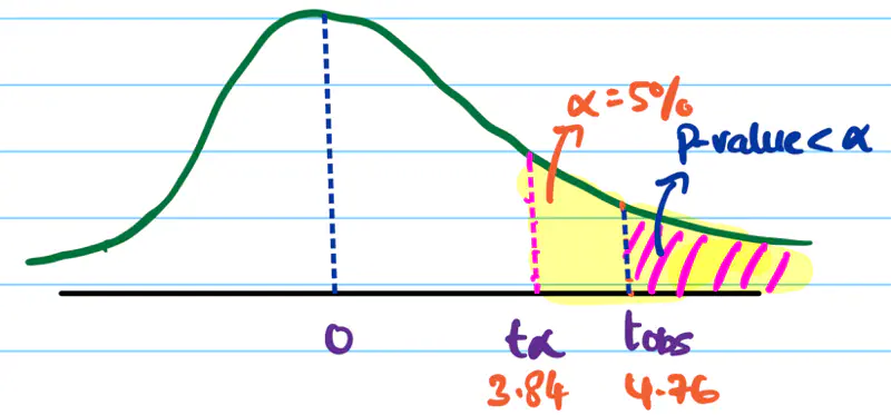
\[ t_{obs} = \chi_{calc}^2 = \sum_{i=1}^2 \frac{(O_i - E_i)^2}{E_i} \\[10pt] = \frac{(62 - 50)^2}{50} + \frac{(38 - 50)^2}{50} \\[10pt] = \frac{144}{50} + \frac{144}{50} \\[10pt] => t_{obs} = 5.76 \]

Since, significance level = 5% = 0.05
Critical value = \(\chi^2(0.05,1)\) = 3.84

Since, \(t_{obs}\) = 5.76 > 3.84 (critical value), we reject the null hypothesis \(H_0\).
Therefore, the coin is biased towards head.

📘

Test of Independence:
It is used to determine whether an association exists between two categorical variables, using a contingency(dependency) table.
It is a non-parametric test, i.e, does NOT make any assumption about the underlying distribution of the data.

Test Statistic:

\[ \chi_{calc}^2 = \sum_{i=1}^R \sum_{i=1}^C \frac{(O_i - E_i)^2}{E_i} \]

\(O_{ij}\): Observed count for \(cell_{i,j}\)
\(E_{ij}\): Expected count for \(cell_{i,j}\), under null hypothesis \(H_0\)
\(R\): Number of rows
\(C\): Number of columns
\(\nu\): Degrees of freedom = (R-1)*(C-1)

Let’s understand the above test statistic in more detail.
We know that, if 2 random variables A & B are independent, then,
\(P(A \cap B) = P(A, B) = P(A)*P(B)\)
i.e Joint Probability = Product of marginal probabilities.

Null Hypothesis \(H_0\): \(A\) and \(B\) are independent.
Alternative Hypothesis \(H_a\): \(A\) and \(B\) are dependent or associated.
N = Sample size
\(P(A_i) \approx \frac{Row ~~ Total_i}{N}\)

\(P(B_j) \approx \frac{Col ~~ Total_j}{N}\)

\(E_{ij}\) : Expected count for \(cell_{i,j}\) = \( N*P(A_i)*P(B_j)\)

=> \(E_{ij}\) = \(N*\frac{Row ~~ Total_i}{N}*\frac{Col ~~ Total_j}{N}\)

=> \(E_{ij}\) = \(\frac{Row ~~ Total_i * Col ~~ Total_j}{N}\)

\(O_{ij}\): Observed count for \(cell_{i,j}\)

💡

A survey of 100 students was conducted to understand whether there is any relation between gender and beverage preference.
Below is the table that shows the number of students who prefer each beverage.

Gender	Tea	Coffee
Male	20	30	50
Female	10	40	50
	30	70

Significance level = 5%

Null Hypothesis \(H_0\): Gender and beverage preference are independent.
Alternative Hypothesis \(H_a\): Gender and beverage preference are dependent.

We know that Expected count for cell(i,j) = \(E_{ij}\) = \(\frac{Row ~~ Total_i * Col ~~ Total_j}{N}\)

\(E_{11} = \frac{50*30}{100} = 15\)

\(E_{12} = \frac{50*70}{100} = 35\)

\(E_{21} = \frac{50*30}{100} = 15\)

\(E_{22} = \frac{50*70}{100} = 35\)

Test Statistic:

\[ t_{obs} = \chi_{calc}^2 = \sum_{i=1}^R \sum_{i=1}^C \frac{(O_i - E_i)^2}{E_i} \\[10pt] = \frac{(20 - 15)^2}{15} + \frac{(30 - 35)^2}{35} + \frac{(10 - 15)^2}{15} + \frac{(40 - 35)^2}{35} \\[10pt] = \frac{25}{15} + \frac{25}{35} + \frac{25}{15} + \frac{25}{35} \\[10pt] => t_{obs} = \frac{50}{15} + \frac{50}{35} \approx 4.76 \]

Degrees of freedom = (R-1)(C-1) = (2-1)(2-1) = 1
Since, significance level = 5% = 0.05
Critical value = \(\chi^2(0.05,1)\) = 3.84

Since, \(t_{obs}\) = 4.76 > 3.84 (critical value), we reject the null hypothesis \(H_0\).
Therefore, the gender and beverage preference are dependent.

Watch Video

End of Section