Hypothesis Testing
8 minute read
Hypothesis Testing is used to determine whether a claim or theory about a population is supported by a sample data,
by assessing whether observed difference or patterns are likely due to chance or represent a true effect.
- It allows companies to test marketing campaigns or new strategies on a small scale before committing to larger investments.
- Based on the results of hypothesis testing, we can make reliable inferences about the whole group based on a representative sample.
- It helps us determine whether an observed result is statistically significant finding, or if it could have just happened by random chance.
It is a statistical inference framework used to make decisions about a population parameter, such as, the mean, variance,
distribution, correlation, etc., based on a sample of data.
It provides a formal method to evaluate competing claims.
Null Hypothesis (\(H_0\)):
Status quo or no-effect or no difference statement; almost always contains a statement of equality.
Alternative Hypothesis (\(H_1 ~or~ H_a\)):
The statement representing an effect, a difference, or a relationship.
It must be true if the null hypothesis is rejected.
- Test of Means:
- 1-Sample Mean Test: Compare sample mean to a known population mean.
- 2-Sample Mean Test: Compare means of 2 populations.
- Paired Mean Test: Compare means when data is paired, e.g., before vs. after test.
- Test of Median:
- Mood’s Median Test
- Sign Test
- Wilcoxon Signed Rank Test (non-parametric)
- Test of Variance:
- Chi-Square Test for a single variance
- F-Test to compare variances of 2 populations
- Test of Distribution(Goodness of Fit):
- Kolmogorov-Smirnov Test
- Shapiro-Wilk Test
- Anderson-Darling Test
- Chi-Square Goodness of Fit Test
- Test of Correlation:
- Pearson’s Correlation Coefficient Test
- Spearman’s Rank Correlation Test
- Kendall’s Tau Correlation Test
- Chi-Square Test of Independence
- Regression Test:
- T-Test: For regression coefficients
- F-Test: For overall regression significance
Step 1: Define the null and alternative hypotheses.
Step 2: Select a relevant statistical test for the task with associated test statistic.
Step 3: Calculate the test statistic under null hypothesis.
Step 4: Select a significance level (\(\alpha\)), i.e, the maximum acceptable false positive rate;
typically - 5% or 1%.
Step 5: Compute the p-value from the observed value of test-statistic.
Step 6: Make a decision to either accept or reject the null hypothesis, based on the significance level (\(\alpha\)).
Say, the data, D: <patient_id, med_1/med_2, recovery_time(in days)>
We need some metric to compare the recovery times of 2 medicines.
We can use the mean recovery time as the metric, because we know that we can use following techniques for comparison:
- 2-Sample T-Test; if \(n < 30\) and population standard deviation \(\sigma\) is unknown.
- 2-Sample Z-Test; if \(n \ge 30\) and population standard deviation \(\sigma\) is known.
Note: Let’s assume the sample size \(n < 30\), because medical tests usually have small sample sizes.
=> We will use the 2-Sample T-Test; we will continue using T-Test throughout the discussion.
Step 1: Define the null and alternative hypotheses.
Null Hypothesis \(H_0\): The mean recovery time of 2 medicines is the same i.e \(Mean_{m1} = Mean_{m2}\) or \(m_{m1} = m_{m2}\).
Alternate Hypothesis \(H_a\): \(m_{m1} < m_{m2}\) (1-Sided T-Test) or \(m_{m1} ⍯ m_{m2}\) (2-Sided T-Test).
Step 2: Select a relevant statistical test for the task with associated test statistic.
Let’s do a 2 sample T-Test, i.e, \(m_{m1} < m_{m2}\)
Step 3: Calculate the test statistic under null hypothesis.
Test Statistic:
For 2 sample T-Test:
s: Standard Deviation
n: Sample Size
Note: If the 2 means are very close then \(t_{obs} \approx 0\).
Step 4: Suppose significance level (\(\alpha\)) = 5% or 0.05.
Step 5: Compute the p-value from the observed value of test-statistic.
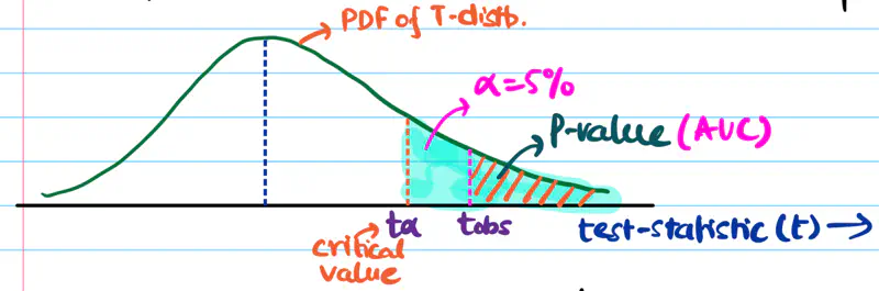
P-Value:
p-value = area under curve = probability of observing test statistic \( \ge t_{obs} \) if the null hypothesis is true.
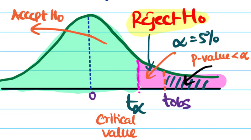
Step 6: Accept or reject the null hypothesis, based on the significance level (\(\alpha\)).
If \(p_{value} < \alpha\), we reject the null hypothesis and accept the alternative hypothesis and vice versa.
Note: In the above example \(p_{value} < \alpha\), so we reject the null hypothesis.
We need to do a left or right sided test, or a 2-sided test, this depends upon our alternate hypothesis and test statistic.
Let’s continue our 2 sample mean T-test to understand the concept:
Left Sided/Tailed Test:
\(H_a\): Mean recovery time of medicine 1 < medicine 2, i.e, \(m_{m_1} < m_{m_2}\)
=> \(m_{m_1} - m_{m_2} < 0\)
Since, the denominator in above equation is always positive.
=> \(t_{obs} < 0\)
Therefore, we need to do a left sided/tailed test.
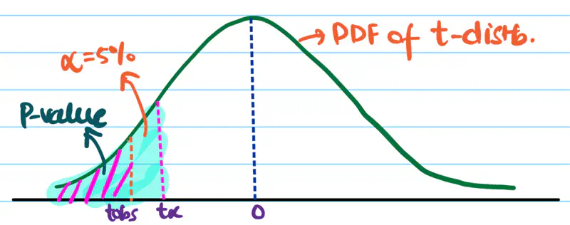
So, we want \(t_{obs}\) to be very negative to confidently conclude that alternate hypothesis is true.
Right Sided/Tailed Test:
\(H_a\): Mean recovery time of medicine 1 > medicine 2, i.e, \(m_{m_1} > m_{m_2}\)
=> \(m_{m_1} - m_{m_2} > 0\)
Similarly, here we need to do a right sided/tailed test.
2 Sided/Tailed Test:
\(H_a\): Mean recovery time of medicine 1 ⍯ medicine 2, i.e, \(m_{m_1} ⍯ ~ m_{m_2}\)
=> \(m_{m_1} - m_{m_2} < 0\) or \(m_{m_1} - m_{m_2} > 0\)
If \(H_a\) is true then \(t_{obs}\) is a large -ve value or a large +ve value.
Since, t-distribution is symmetric, we can divide the significance level \(\alpha\) into 2 equal parts.
i.e \(\alpha = 2.5\%\) on each side.
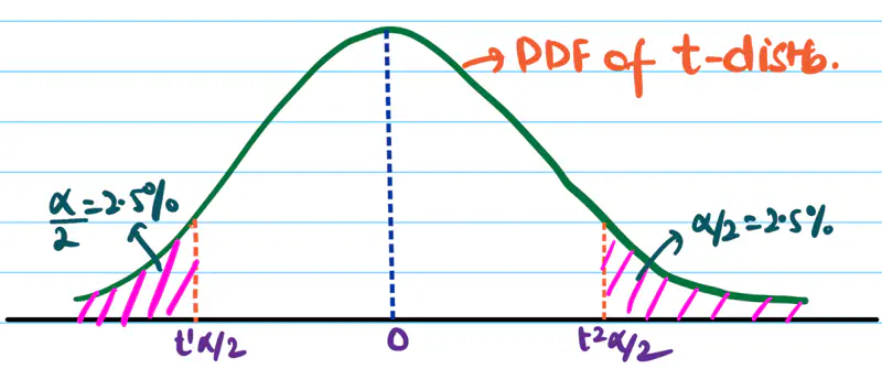
So, we want \(t_{obs}\) to be very negative or very positive to confidently conclude that the alternate hypothesis is true. We accept \(H_a\) if \(t_{obs} < t^1_{\alpha/2}\) or \(t_{obs} > t^2_{\alpha/2}\).
Note: For critical applications ‘\(\alpha\)’ can be very small i.e. 0.1% or 0.01%, e.g medicine.
It is the probability of wrongly rejecting a true null hypothesis, known as a Type I error or false +ve rate.
- Tolerance level of wrongly accepting alternate hypothesis.
- If the p-value < \(\alpha\), we reject the null hypothesis and conclude that the finding is statistically NOT so significant..
It is a specific point on the test-statistic distribution that defines the boundaries of the null hypothesis
acceptance/rejection region.
It tells us that at what value (\(t_{\alpha}\)) of test statistic will the area under curve be equal to the significance level \(\alpha\).
For a right tailed/sided test:
- if \(t_{obs} > t_{\alpha} => p_{value} < \alpha\); therefore, reject null hypothesis.
- if \(t_{obs} < t_{\alpha} => p_{value} \ge \alpha\); therefore, failed to reject null hypothesis.
It is the probability that a hypothesis test will correctly reject a false null hypothesis (\(H_{0}\)) when the alternative hypothesis (\(H_{a}\)) is true.
Power of test = \(1 - \beta\)
Probability of correctly accepting alternate hypothesis (\(H_{a}\))
\(\alpha\): Probability of wrongly accepting alternate hypothesis \(H_{a}\)
\(\beta\): Probability of wrongly rejecting alternate hypothesis \(H_{a}\)

Yes, having a large sample size makes a hypothesis test more powerful.
- As n increases, sample mean \(\bar{x}\) approaches the population mean \(\mu\).
- Also, as n increases, t-distribution approaches normal distribution.
It is a standardized objective measure that complements p-value by clarifying whether a statistically significant
finding has any real world relevance.
It quantifies the magnitude of relationship between two variables.
- Larger effect size => more impactful effect.
- Standardized (mean centered + variance scaled) measure allows us to compare the imporance of effect across various studies or groups, even with different sample sizes.
Effect size is measured using Cohen’s d formula:
\(\bar{X}\): Sample mean
\(s_p\): Pooled Standard deviation
\(n\): Sample size
\(s\): Standard deviation
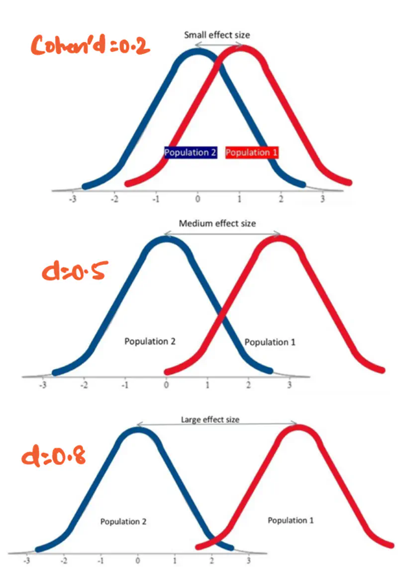
Note: Theoretically, Cohen’s d value can range from negative infinity to positive infinity.
but for practical purposes, we use the following value:
small effect (\(d=0.2\)), medium effect (\(d=0.5\)), and large effect (\(d\ge 0.8\)).
More overlap => less effect i.e low Cohen’s d value.
- A study on drug trials finds that patients taking a new drug had statistically significant
improvement (p-value<0.05), compared to a placebo group.
- Small effect size: Cohen’s d = 0.1 => drug had minimal effect.
- Large effect size: Cohen’s d = 0.8 => drug produced substantial improvement.
End of Section