Performance Metrics

📘 Performance Metrics:
They are quantitative measures used to evaluate how well a machine learning model performs on unseen data.
E.g.: For regression models, we have - MSE, RMSE, MAE, R^2 metric, etc.
Here, we will discuss various performance metrics for classification models.

📘

Confusion Matrix:
It is a table that summarizes model’s predictions against the actual class labels, detailing where the model succeeded and where it failed.
It is used for binary or multi-class classification problems.

	Predicted Positive	Predicted Negative
Actual Positive	True Positive (TP)	False Negative (FN)
Actual Negative	False Positive (FP)	True Negative (TN)

Type-1 Error:
It is the number of false positives.
e.g.: Model predicted that a patient has diabetes, but the patient actually does NOT have diabetes; “false alarm”.

Type-2 Error:
It is the number of false negatives. e.g.: Model predicted that a patient does NOT have diabetes, but the patient actually has diabetes; “a miss”.

💡

Analyze the performance of an access control system. Below is the data for 1000 access attempts.

	Predicted Authorised Access	Predicted Unauthorised Access
Actual Authorised Access	90 (TP)	10 (FN)
Actual Unauthorised Access	1 (FP)	899 (TN)

\[ Precision = \frac{TP}{TP + FP} = \frac{90}{90 + 1} \approx 0.989 \]

When the system allows access, it is correct 98.9% of the time.

\[ Recall = \frac{TP}{TP + FN} = \frac{90}{90 + 10} = 0.9 \]

The system caught 90% of all authorized accesses.

\[ F1 ~ Score = 2 * \frac{Precision \times Recall}{Precision + Recall} \\[10pt] = 2 * \frac{0.989 \times 0.9}{0.989 + 0.9} \\[10pt] => F1 ~ Score \approx 0.942 \]

📘

Receiver Operating Characteristic (ROC) Curve:
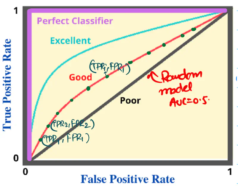
It is a graphical plot that shows the discriminating ability of a binary classifier system, as its discrimination threshold is varied.
Y-axis: True Positive Rate (TPR), Recall, Sensitivity
\(TPR = \frac{TP}{TP + FN}\)

X-axis: False Positive Rate (FPR); (1 - Specificity)
\(FPR = \frac{FP}{FP + TN}\)

Note: A binary classifier model outputs a probability score between 0 and 1.
and a threshold (default=0.5) is applied to the probability score to get the final class label.
\(p \ge 0.5\) => Positive Class
\(p < 0.5\) => Negative Class

Algorithm:

1. Sort the data by the probability score in descending order.
   
2. Set each probability score as the threshold for classification and calculate the TPR and FPR for each threshold.
   
3. Plot each pair of (TPR, FPR) for all ’n’ data points to get the final ROC curve.
   

e.g.:

Patient_Id	True Label \(y_i\)	Predicted Probability Score \(\hat{y_i}\)
1	1	0.95
2	0	0.85
3	1	0.72
4	1	0.63
5	0	0.59
6	1	0.45
7	1	0.37
8	0	0.20
9	0	0.12
10	0	0.05

Set the threshold \(\tau_1\) = 0.95, calculate \({TPR}_1, {FPR}_1\)
Set the threshold \(\tau_2\) = 0.85, calculate \({TPR}_2, {FPR}_2\)
Set the threshold \(\tau_3\) = 0.72, calculate \({TPR}_3, {FPR}_3\)
…
…
Set the threshold \(\tau_n\) = 0.05, calculate \({TPR}_n, {FPR}_n\)

Now, we have ’n’ pairs of (TPR, FPR) for all ’n’ data points.
Plot the points on a graph to get the final ROC curve.

AU ROC = AUC = Area under the ROC curve = Area under the curve

Note:

1. If AUC < 0.5, then invert the labels of the classes.
2. ROC does NOT perform well on imbalanced data.
   • Either balance the data or
   • Use Precision-Recall curve.

💡 What is the AUC of a random binary classifier model?

AUC of a random binary classifier model = 0.5
Since, labels are randomly generated as 0/1 for binary classification, so 50% labels from each class.
Because random number generators generate numbers uniformly in the given range.

💡 Why ROC can be misleading for imbalanced data ?

Let’s understand this with the below fraud detection example.
Below is a dataset from a fraud detection system for N = 10,000 transactions.
Fraud = 100, NOT fraud = 9900

	Predicted Fraud	Predicted NOT Fraud
Actual Fraud	80 (TP)	20 (FN)
Actual NOT Fraud	220 (FP)	9680 (TN)

\[TPR = \frac{TP}{TP + FN} = \frac{80}{80 + 20} = 0.8\]

\[FPR = \frac{FP}{FP + TN} = \frac{220}{220 + 9680} \approx 0.022\]

If we check the location of above (TPR, FPR) pair on the ROC curve, then we can see that it is very close to the top-left corner.
This means that the model is very good at detecting fraudulent transactions, but that is NOT the case.
This is happening because of the imbalanced data, i.e, count of NOT fraud transactions is 99 times of fraudulent transactions.

Let’s look at the Precision value:

\[Precision = \frac{TP}{TP + FP} = \frac{80}{80 + 220} = \frac{80}{300}\approx 0.267\]

We can see that the model has poor precision,i.e, only 26.7% of flagged transactions are actual frauds.
Unacceptable precision for a good fraud detection system.

📘

Precision-Recall Curve:
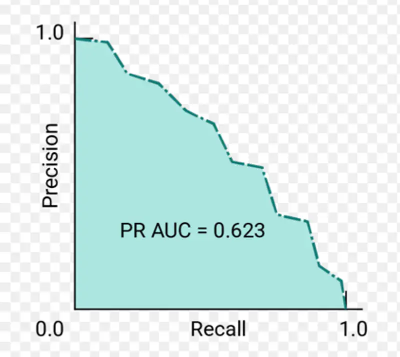
It is used to evaluate the performance of a binary classifier model across various thresholds.
It is similar to the ROC curve, but it uses Precision instead of TPR on the Y-axis.
Plots Precision (Y-axis) against Recall (X-axis) for different classification thresholds.
Note: It is useful when the data is imbalanced.

\[ Precision = \frac{TP}{TP + FP} \\[10pt] Recall = \frac{TP}{TP + FN} \]

AU PRC = PR AUC = Area under Precision-Recall curve

Let’s revisit the fraud detection example discussed above to understand the utility of PR curve.

	Predicted Fraud	Predicted NOT Fraud
Actual Fraud	80 (TP)	20 (FN)
Actual NOT Fraud	220 (FP)	9680 (TN)

\[Precision = \frac{TP}{TP + FP} = \frac{80}{80 + 220} = \frac{80}{300}\approx 0.267\]

\[Recall = \frac{TP}{TP + FN} = \frac{80}{80 + 20} = \frac{80}{100}\approx 0.8\]

If we check the location of above (Precision, Recall) point on PRC curve, we will find that it is located near the bottom right corner, i.e, the model performance is poor.