Z-Test
7 minute read
It is a statistical test used to determine whether there is a significant difference between mean of 2 groups or sample and population mean.
- It is a parametric test, since it assumes data to be normally distributed.
- Appropriate when:
- sample size \(n \ge 30\).
- population standard deviation \(\sigma \) is known.
- It is based on Gaussian/normal distribution.
- It compares the difference between means relative to standard error, i.e, standard deviation of sampling distribution of sample mean.
There are 2 types of Z-Test:
- 1-Sample Z-Test: Used to compare the mean of a sample mean with a population mean.
- 2-Sample Z-Test: Used to compare the sample means of 2 independent samples.
It is a standardized score that measures how many standard deviations a particular data point is away from the population mean \(\mu\).
- Transform a normal distribution \(\mathcal{N}(\mu, \sigma^2)\) to a standard normal distribution \(Z \sim \mathcal{N}(0, 1)\).
- Standardized score helps us compare values from different normal distributions.
Z-score is calculated as:
\[Z = \frac{x - \mu}{\sigma}\]x: data point
\(\mu\): population mean
\(\sigma\): population standard deviation
e.g:
- Z-score of 1.5 => data point is 1.5 standard deviations above the mean.
- Z-score of -2.0 => data point is 2.0 standard deviations below the mean.
Z-score helps to define probability areas:
- 68% of the data points fall within \(\pm 1 \sigma\).
- 95% of the data points fall within \(\pm 2 \sigma\).
- 99.7% of the data points fall within \(\pm 3 \sigma\).
Note:
- Z-Test applies the concept of Z-score to sample mean rather than a single data point.
It is used to test whether the sample mean \(\bar{x}\) is significantly different from a known population mean \(\mu\).
Test Statistic:
\(\bar{x}\): sample mean
\(\mu\): hypothesized population mean
\(\sigma\): population standard deviation
\(n\): sample size
\(\sigma / \sqrt{n}\): standard error of mean
Read more about Standard Error
Note: Test statistic Z follows a standard normal distribution \(Z \sim \mathcal{N}(0, 1)\).
It is used to test whether the sample means \(\bar{x_1}\) and \(\bar{x_2}\) of 2 independent samples are significantly different from each other.
Test Statistic:
\(\bar{x_1}\): sample mean of first sample
\(\bar{x_2}\): sample mean of second sample
\(\sigma_1\): population standard deviation of first sample
\(\sigma_2\): population standard deviation of second sample
\(n_1\): sample size of first sample
\(n_2\): sample size of second sample
Note: Test statistic Z follows a standard normal distribution \(Z \sim \mathcal{N}(0, 1)\).
After applying a new optimisation, and n=100 runs, yields a sample mean of 117 seconds.
Does the optimisation significantly reduce the runtime of the model?
Consider the significance level of 5%.
Null Hypothesis: \(\mu = 120\) seconds, i.e, no change.
Alternative Hypothesis: \(\mu < 120\) seconds => left tailed test.
We will use 1-sample Z-Test to test the hypothesis.
Test Statistic:
Since, significance level \(\alpha\) = 5% =0.05.
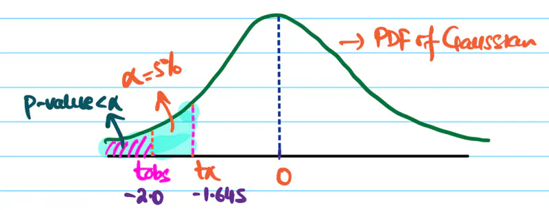
Critical value \(Z_{0.05}\) = -1.645
Important: Find the value of \(Z_{\alpha}\) in Z-Score Table

Our \(t_{obs}\) is much more extreme than the the critical value \(Z_{0.05}\), => p-value < 5%.
Hence, we reject the null hypothesis.
Therefore, there is a statistically significant evidence that the new optimisation reduces the runtime of the model.
It is a statistical hypothesis test used to determine if there is a significant difference between the proportion
of a characteristic in two independent samples or to compare a sample proportion to a known population value
- It is used when dealing with categorical data, such as, success/failure, male/female, yes/no etc.
It is of 2 types:
- 1-Sample Z-Test of Proportion: Used to test whether the observed proportion in a sample differs from hypothesized proportion.
- 2-Sample Z-Test of Proportion: Used to compare whether the 2 independent samples differ in their proportions.
The categorical data,i.e success/failure, is discrete that can be modeled as Bernoulli distribution.
Let’s understand how this Bernoulli random variable can be approximated as a Gaussian distribution for a very large sample size,
using Central Limit Theorem.
Read more about Central Limit Theorem
Note:We will not prove the complete thing, but we will understand the concept in enough depth for clarity.
\(Y \sim Bernoulli(p)\)
\(X \sim Binomial(n,p)\)
E[X] = mean = np
Var[X] = variance = np(1-p)
X = total number of successes
p = true probability of success
n = number of trials
Proportion of Success in sample = Sample Proportion = \(\hat{p} = \frac{X}{n}\)
e.g.: If n=100 people were surveyed, and 40 said yes, then \(\hat{p} = \frac{40}{100} = 0.4\)
By Central Limit Theorem, we can state that for very large ’n’ Binomial distribution’s mean and variance can be used as an
approximation for Gaussian/Normal distribution:
Since, \(\hat{p} = \frac{X}{n}\)
We can say that:
Mean = \(\mu_{\hat{p}} = p\) = True proportion of success in the entire population
Standard Error = \(SE_{\hat{p}} = \sqrt{Var[\frac{X}{n}]} = \sqrt{\frac{p(1-p)}{n}}\) = Standard Deviation of the sample proportion
Note: Large Sample Condition - Approximation is only valid when the expected number of successes and failures are both > 10 (sometimes 5).
\(np \ge 10 ~and~ n(1-p) \ge 10\)
It is used to test whether the observed proportion in a sample differs from hypothesized proportion.
\(\hat{p} = \frac{X}{n}\): Proportion of success observed in a sample
\(p_0\): Specific propotion value under the null hypothesis
\(SE_0\): Standard error of sample proportion under the null hypothesis
Z-Statistic: Measures how many standard errors is the observed sample proportion \(\hat{p}\) away from \(p_0\)
Test Statistic:
It is used to compare whether the 2 independent samples differ in their proportions.
- Standard test used in A/B testing.
A company wants to compare its 2 different website designs A & B.
Below is the table that shows the data:
| Design | # of visitors(n) | # of signups(x) | conversion rate(\(\hat{p} = \frac{x}{n}\)) |
|---|---|---|---|
| A | 1000 | 80 | 0.08 |
| B | 1200 | 114 | 0.095 |
Is the design B better, i.e, design B increases conversion rate or proportion of visitors who sign up?
Consider the significance level of 5%.
Null Hypothesis: \(\hat{p_A} = \hat{p_B}\), i.e, no difference in conversion rates of 2 designs A & B.
Alternative Hypothesis: \(\hat{p_B} > \hat{p_A}\) i.e conversion rate of B > A => right tailed test.
Check large sample condition for both samples A & B.
\(n\hat{p_A} = 80 > 10 ~and~ n(1-\hat{p_A}) = 920 > 10\)
Similarly, we can show for B too.
Pooled proportion:
\[ \bar{p} = \frac{x_A+x_B}{n_A+n_B} = \frac{80+114}{1000+1200} = \frac{194}{2200} \\[10pt] => \bar{p}\approx 0.0882 \]Standard Error(Pooled):
\[ SE=\sqrt{\bar{p}(1-\bar{p})(\frac{1}{n_1} +\frac{1}{n_2})} \\[10pt] = \sqrt{0.0882(1-0.0882)(\frac{1}{1000} +\frac{1}{1200})} \\[10pt] => SE \approx 0.0123 \]Test Statistic(Z):
\[ t_{obs} = \frac{\hat{p_B}-\hat{p_A}}{SE_{\hat{p_A}-\hat{p_B}}} \\[10pt] = \frac{0.095-0.0882}{0.0123} \\[10pt] => t_{obs} \approx 1.22 \]Significance level \(\alpha\) = 5% =0.05.
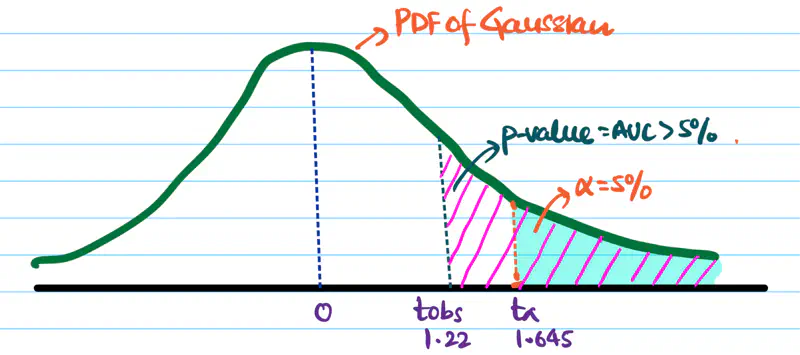
Critical value \(Z_{0.05}\) = 1.645

Since, \(t_{obs} < Z_{0.05}\) => p-value > 5%.
Hence, we fail to reject the null hypothesis.
Therefore, the observed conversion rate of design B is due to random chance; thus, B is not a better design.
End of Section