GRU
5 minute read
LSTMs are complex, which makes them slower to train and more computationally intensive.
- three gates (forget, input, output) and many parameters.
- separate long-term memory (cell state) and short term memory (hidden state).
GRU is simplified LSTM with fewer gates, fewer parameters and simpler architecture, while retaining the ability to capture long-term dependencies, often leading to faster training times and reduced computational costs.
- Simpler Architecture:
- GRU has two gates (reset, update) instead of three.
- This reduces the number of weight matrices by roughly 25-33%, leading to faster training and lower memory consumption.
- Structural Simplicity:
- By merging the “Cell State” (\(C_t\)) and “Hidden State” (\(h_t\)) into a single vector, it eliminates the redundant storage of information.
- Performance on Small Data:
- Due to fewer parameters, GRUs are often less prone to overfitting than LSTMs when training on smaller datasets.
GRU Memory Cell
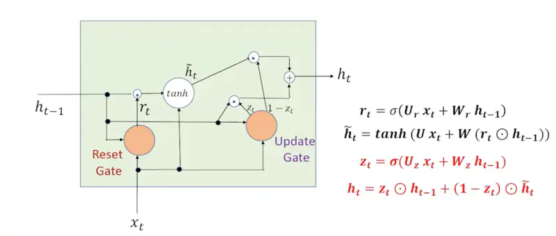
GRU Architecture
- Each gate in an GRU functions as a single-layer feedforward neural network that lives inside the GRU cell.
- Each gate has its own unique, learnable weight matrices (\(W\)) and bias vectors (\(b\)).
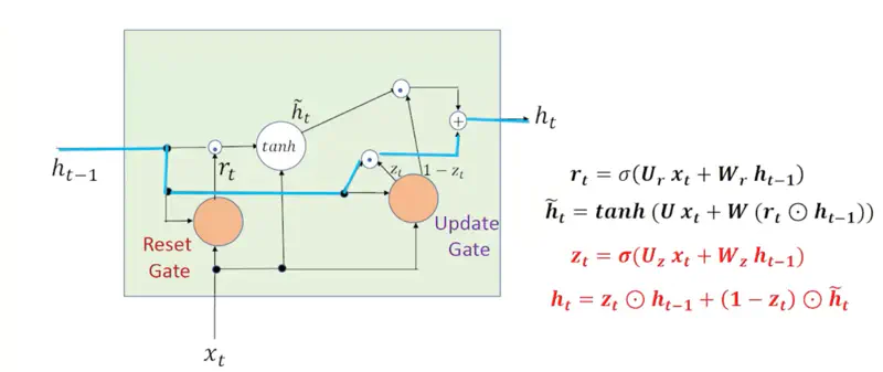
Decides how much of the past hidden state (\(h_{t-1}\)) is relevant to calculating the current candidate.
\[r_t = \sigma(U_r x_t + W_r h_{t-1} + b_r)\]- \(r_t = 0\): “forget” the past context entirely.
- \(r_t = 1\): use everything from the past.
Read more about Vector Operations
Read more about Activation Function
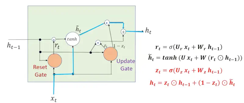
This is the “suggestion” for what the new state should look like.
\[\tilde{h}_t = \tanh(U x_t + W(r_t \odot h_{t-1}) + b_h)\]Note: If \(r_t=0\), then \(r_t \odot h_{t-1}\) will wipe out the previous state completely.
Read more about Vector Operations
Read more about Activation Function
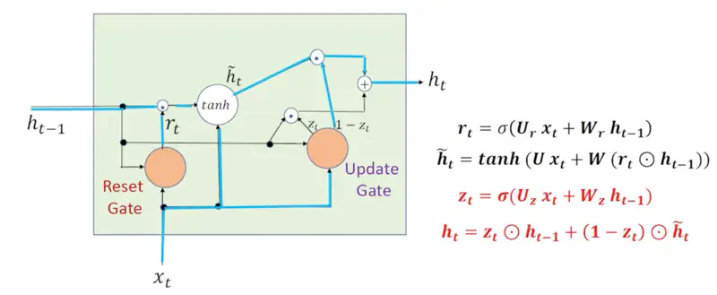
Performs a linear interpolation (slider) between the old state and the new suggestion.
\[z_t = \sigma(U_z x_t + W_z h_{t-1} + b_z)\]Final state:
\[h_t = \underbrace{z_t \odot h_{t-1}}_{\text{Keep\ the\ Old}} + \underbrace{(1 - z_t) \odot \tilde{h}_t}_{\text{Adopt\ the\ New}} \]Read more about Vector Operations
Read more about Activation Function
- Sigmoid (Gates): Outputs 0 to 1;
- For “gating” (blocking or passing info).
- Tanh (Candidate): Outputs -1 to 1;
- Allows the candidate to either add to the memory (positive values) or subtract/correct the memory (negative values).
- Element Wise Product: \[ \mathbf{a} \odot \mathbf{b} = \begin{bmatrix} a_1 \\ a_2 \\ \vdots \\ a_n \end{bmatrix} \odot \begin{bmatrix} b_1 \\ b_2 \\ \vdots \\ b_n \end{bmatrix} = \begin{bmatrix} a_1 b_1 \\ a_2 b_2 \\ \vdots \\ a_n b_n \end{bmatrix} \]
Gates Summary
| Component | Role |
|---|---|
| Reset Gate | “Clear the cache for a new sub-topic.” |
| Candidate | Propose new state. |
| Update Gate | Mix old + new info. |
Now let’s understand how back propagation through time happens in GRU.
It is similar to LSTM as GRU is also sequential in nature and processes words in a sentence one by one.
- Hidden State = \(h_t = z_t \odot h_{t-1} + (1 - z_t) \odot \tilde{h}_t\)
- Gradient = \(\frac{\partial h_t}{\partial h_{t-1}} = z_t + (1-z_t)(W.r_t.tanh')\)
Recursively (for all words at different time steps): \[ \frac{\partial h_t}{\partial h_{k}} = \prod_{i=k+1}^t z_i + (1-z_i)(W.r_i.tanh')\]
Therefore, in GRU , the gradient is mostly determined by \(z_t\).
- If the information is important then the network sets the \(z_t = 1\).
- This means the gradient can flow backwards through hundreds of time steps without being scaled down to zero.
Note: Therefore, unlike RNNs, the vanishing/exploding gradient problem is significantly reduced in GRU, because of the stable gradient flow, allowing GRU to learn long range dependencies.
In RNN, the gradient is given by:
\[ \frac{\partial E_t}{\partial h_k } = \delta_t \prod_{i=k+1}^t \sigma'(a_i).W \propto \prod \text{Activation Gradient x Weight} \]Read more about Back Propagation Through Time in RNN
Read more about Vanishing Gradient Problem
First of all let us understand what is the meaning of “Carousel”.
Carousel 🎠 is a rotating circular amusement ride with seats (often horses) commonly called a merry-go-round, or a circular conveyor system.
And, now let us understand the meaning of Constant Error Carousel.
If we place a “message” (the gradient) on a horse, and the carousel rotates with no friction or resistance (\(f_t=1\)), the information keeps circulating exactly as it is for an infinite number of rotations.
In other words, if the forget get output for a word is set to 1, then the model does not forget it even if there are infinite number words before it till the beginning of the sentence, i.e, no vanishing gradient problem.
Let us understand how GRU works with the help of few examples.
1. Context Shift
Say, there is a context shift between sentences, i.e, say , the previous sentence discussed ‘Stars’
and in the current sentence we start discussing “Fish”.
Clearly, there is a context shift, and we want to the network to forget the previous context entirely and start fresh.
In that case \(r_t=0, ~ z_t=0 \), so that the current input ‘\(x_t\)’ is passed as it is.
2. Ignore Current Input
Say, we have a GRU processing a long review to determine sentiment:
“The phone I bought yesterday, despite having a slightly scratched screen that makes it annoying to use sometimes, is absolutely amazing and has a black charger.”
- The model reads “absolutely amazing” and updates its hidden state to a strong positive sentiment.
- Later the review adds irrelevant details like - “has a black charger”,
- so GRU learns to set \(z_t \approx 1\) when these words are processed, and ignores them.
Note: When GRU wants to ignore current input to preserve long-term memory, it sets \(z_t\) close to 1.
3. Default Behavior (RNN)
GRU isn’t trying to store long-term memories; it is simply processing the current input \(x_t\)
in the context of the immediately preceding hidden state \(h_{t-1}\).
- Reset Gate \(r_t = 1\): The candidate hidden state \(\tilde{h_{t}}\) has full access to the previous hidden state (\(h_{t-1}\)).
- Nothing from the past is blocked.
- Update Gate (\(z_t = 0\)): The network decides to entirely replace the old state with the new candidate state.
Note: GRU essentially “forgets” the past and behaves like a standard Simple RNN.