LSTM
4 minute read
RNNs are not good at capturing long range dependencies (due to vanishing gradient problem).

By the time the RNN is processing “not entertaining” it forgets the subject, i.e, “Jurassic Park movie” because they are separated too far.
LSTM solves vanishing gradient problem by introducing:
- Cell State (\(C_t\)): which acts as a “long-term” memory conveyor belt that runs parallel to the
- Hidden State (\(h_t\)): the “short-term” working memory (similar to RNN)
LSTM Memory Cell
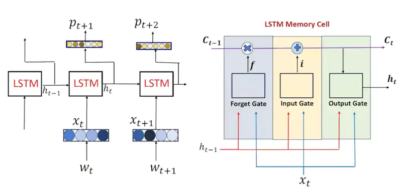
LSTM Architecture
- Each gate in an LSTM functions as a single-layer feedforward neural network that lives inside the LSTM cell.
- Each gate has its own unique, learnable weight matrices (\(W\)) and bias vectors (\(b\)).
Decides what information from the previous cell state (\(C_{t-1}\)) is no longer useful and should be discarded.
\[f_t = \sigma(W_f \cdot [h_{t-1}, x_t] + b_f)\]- \(f_t = 0\): “forget” the previous memory entirely.
- \(f_t = 1\): “remember” everything.
Read more about Vector Operations
Read more about Activation Function
This stage decides what new information will be stored in the cell state (\(C_t\)).
- Input Gate: Decides which values to update. \[ i_t = \sigma(W_i \cdot [h_{t-1}, x_t] + b_i) \]
- Candidates: Creates a vector of new candidate values that could be added to the state. \[\tilde{C}_t = \tanh(W_C \cdot [h_{t-1}, x_t] + b_C)\]
- Update the Cell State: This is the “memory update” where the old memory is scaled by the forget gate and the new information is scaled by the input gate. \[C_t = \underbrace{f_t \odot C_{t-1}}_{\text{Filtered\ Old\ Info}} + \underbrace{i_t \odot \tilde{C}_t}_{\text{Filtered\ New\ Info}}\]
Read more about Vector Operations
Read more about Activation Function
Determines the next hidden state (\(h_t\)).
\[o_t = \sigma(W_o \cdot [h_{t-1}, x_t] + b_o) \]\[h_t = o_t \odot \tanh(C_t)\]This ‘\(h_t\)’ is used for predictions and as input for the next time step.
Read more about Vector Operations
Read more about Activation Function
- Sigmoid (Gates): Outputs 0 to 1;
- For “gating” (blocking or passing info).
- Tanh (Candidate): Outputs -1 to 1;
- Allows the candidate to either add to the memory (positive values) or subtract/correct the memory (negative values).
- Element Wise Product: \[ \mathbf{a} \odot \mathbf{b} = \begin{bmatrix} a_1 \\ a_2 \\ \vdots \\ a_n \end{bmatrix} \odot \begin{bmatrix} b_1 \\ b_2 \\ \vdots \\ b_n \end{bmatrix} = \begin{bmatrix} a_1 b_1 \\ a_2 b_2 \\ \vdots \\ a_n b_n \end{bmatrix} \]
Gates Summary
| Component | Role |
|---|---|
| Forget Gate | Decide which information to delete. |
| Input Gate | Decide which information to add. |
| Candidate | Actual new information. |
| Cell State | Long-term memory; conveyor belt. |
| Output Gate | Decide the next hidden state (short-term memory). |
Now let’s understand how back propagation through time happens in LSTM.
It is similar to RNN as LSTM is also sequential in nature and processes words in a sentence one by one.
- Cell State = \(C_t = f_t \odot C_{t-1} + i_t \odot \tilde{C}_t\)
- Gradient = \(\frac{\partial c_{t} } {\partial c_{t-1}} = f_t\)
- Recursively (for all words at different time steps): \[ \frac{\partial c_{t} } {\partial c_{k}} = \prod_{i=k+1}^t f_i\]
Therefore, in LSTM , the gradient is determined by the forget gate \(f_t\).
- If the information is important then the network sets the \(f_t = 1\).
- This means the gradient can flow backwards through hundreds of time steps without being scaled down to zero.
Note: Therefore, unlike RNNs, the vanishing/exploding gradient problem is significantly reduced in LSTM, because of the stable gradient flow, allowing LSTM to learn long range dependencies.
In RNN, the gradient is given by:
\[ \frac{\partial E_t}{\partial h_k } = \delta_t \prod_{i=k+1}^t \sigma'(a_i).W \propto \prod \text{Activation Gradient x Weight} \]Read more about Back Propagation Through Time in RNN
Read more about Vanishing Gradient Problem
First of all let us understand what is the meaning of “Carousel”.
Carousel 🎠 is a rotating circular amusement ride with seats (often horses) commonly called a merry-go-round, or a circular conveyor system.
And, now let us understand the meaning of Constant Error Carousel.
If we place a “message” (the gradient) on a horse, and the carousel rotates with no friction or resistance (\(f_t=1\)), the information keeps circulating exactly as it is for an infinite number of rotations.
In other words, if the forget get output for a word is set to 1, then the model does not forget it even if there are infinite number words before it till the beginning of the sentence, i.e, no vanishing gradient problem.