Recurrent Neural Network
7 minute read
N-gram model is a probabilistic tool used to predict the next item in such a sequence by looking at the previous \(n-1\) items.
The “n” in n-gram refers to the number of items in the sequence.
- Unigram (\(n=1\)): Single words (e.g., “We”, “learn”, “RNN”).
- Bigram (\(n=2\)): Pairs of consecutive words (e.g., “We learn”, “learn RNN”).
- Trigram (\(n=3\)): Triplets of consecutive words (e.g., “We learn RNN”)
Limitation
Natural language text may not be of fixed size.
Every sentence is of different length.
We cannot use n-gram model, because it calculates the probability of a word based on the ‘\(n-1\)’ preceding words, relying only on a fixed, finite context window.
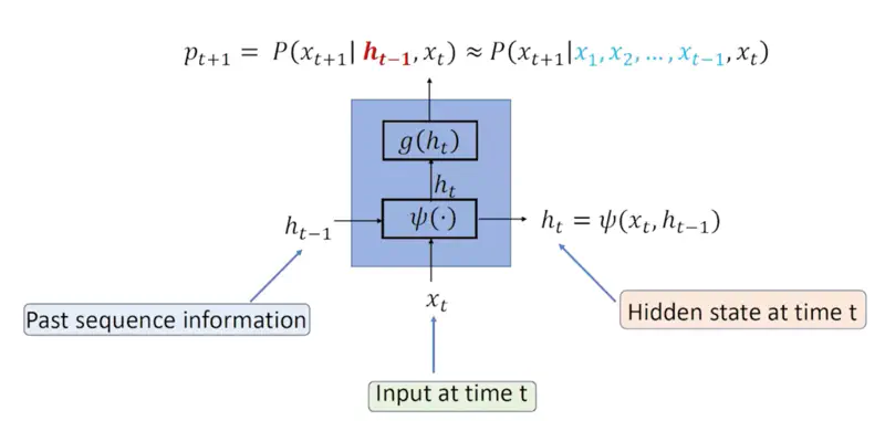
So, we need a model that can process an input of any length and use all the sequence information from the past.
At each step, the RNN maintains a “hidden state” that captures information about the words seen so far.
Recurrent Relation
\[P(x_{t+1} | x_1, x_2, \dots, x_t) \approx P(x_{t+1} | h_{t-1}, x_t)\]\(h_{t-1}\): Hidden/latent vector that captures all the information seen till time instance ‘\(t-1\)’.
Note: Hidden state can theoretically capture information from the entire history of the sequence.
RNN Architecture
RNN Parameters
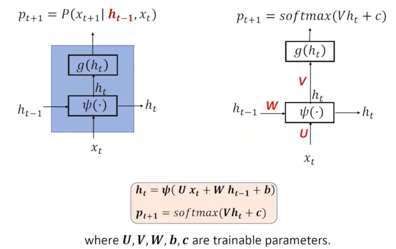
Note: Number of parameters is independent of input sequence length, because the same neural network is processing different words at different time stamps.
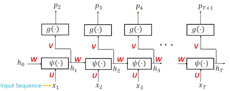
Sequence Information
See below how different words are input at different time stamps and the hidden state stores the sequence information seen till that time stamp.
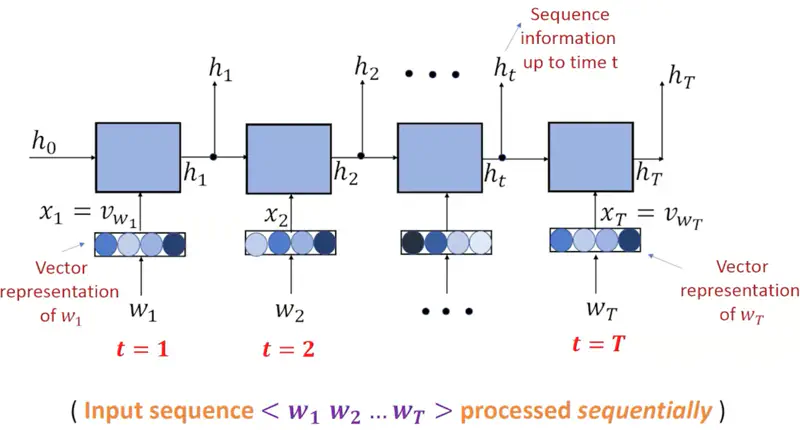
Note: The input \(x_1, x_2, \dots, x_T \) are the vector representations of the words or word embeddings, earlier OHE was used, but after 2013, Word2Vec or GloVe etc. are mostly used.
Teacher Forcing
Say we are training the RNN model for text generation or language modeling,
i.e, we predict the next word based on all the words seen in the past.
e.g. Let’s assume that we are using the following sentence to train the model:
“This is a cat.”
Now at time ’t’ the model sees the current word (\(w_t\)) “a” and tries to predict the “t+1” or next word.
It generates a probability distribution (softmax output) \(p_{t+1}\) of all the words in the vocabulary.
But the model has just started training, and it has no idea of sentences now, so it can predict any garbage value,
which may be totally meaningless.
So, in order to train the model and learn the patterns from the training data instead of feeding the predicted word \(p_{t+1}\)
as the next input i.e \(w_{t+1}\), we feed the actual word i.e “cat” as \(w_{t+1}\).
This is called Teacher Forcing.
Note: This stops the error (caused by predicting some garbage value during training) from being propagated through the network.
RNN Algorithm
- For every sentence ‘i’ in the corpus:
- For every token ‘t’ in the sentence:
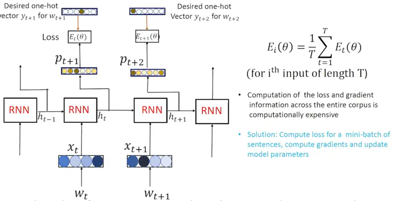
- Compute probability distribution \(p_t\) on the vocabulary, given the previous ‘t-1’ words in the sentence.
- Compute the loss (cross entropy) between \(p_t\) and \(y_t\) (desired OHE). \[ E_t(\theta) = - \sum_{j=1}^{|V|} y_{t,j} ~ \text{log}(p_{t,j}) \]
- Compute the average overall training loss for the sentence ‘i’. \[ E_i(\theta) = \frac{1}{T} \sum_{t=1}^{T} E_t(\theta) \]
- For every token ‘t’ in the sentence:
- Compute gradient information using back propagation through time and update model parameters.
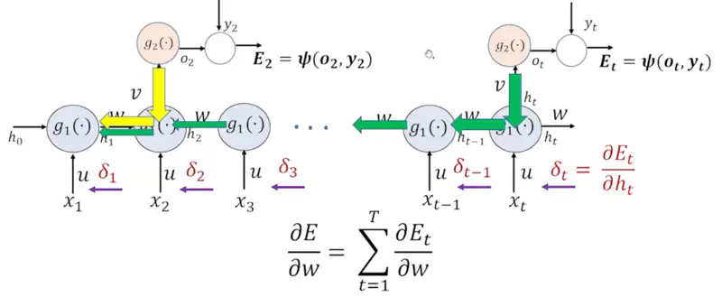
Calculate the error at each time step and propagate it backward to update RNN weights.
Forward Pass
- \(a_t = Ux_t + Wh_{t-1} + b\)
- \(h_t = \sigma(a_t) = \sigma(Ux_t + Wh_{t-1} + b)\), (activation function = sigmoid, tanh, ReLU etc.)
- \(o_t = Vh_t + c\)
- \(p_{t+1} = \text{softmax} (o_t)\)
- \(E_t = \psi(o_t, y_t)\), (cross -entropy loss)
Derivative of Error wrt to weight:
\[\frac{\partial E}{\partial w } = \sum_{t=1}^T \frac{\partial E_t}{\partial w }\]We can re-write it using the chain rule of differentiation:
\[\frac{\partial E}{\partial w } = \sum_{t=1}^T \frac{\partial E_t}{\partial h_t } \frac{\partial h_t}{\partial w }\]Let, \(\delta_t = \frac{\partial E_t}{\partial h_t }\)
Similarly, error at ‘k-th’ hidden state:
\[\frac{\partial E_t}{\partial h_k } = \frac{\partial E_t}{\partial h_t }. \frac{\partial h_{t} } {\partial h_{t-1} }. \frac{\partial h_{t-1} }{\partial h_{t-2} } \dots \frac{\partial h_{k+1} } {\partial h_k }\]\[\implies \frac{\partial E_t}{\partial h_k } = \delta_t \prod_{i=k+1}^t \frac{\partial h_{i} } {\partial h_{i-1} }\]Let’s calculate \(\frac{\partial h_{t} } {\partial h_{t-1}}\) now:
\[\frac{\partial h_{t} } {\partial h_{t-1}} = \frac{\partial h_{t} } {\partial a_{t}}. \frac{\partial a_{t} } {\partial h_{t-1}}\]\[ \because h_t = \sigma(a_t)\]\[ \tag{1} \implies \frac{\partial h_{t} } {\partial a_{t}} = \sigma'(a_t) \]\[\because a_t = Ux_t + Wh_{t-1} + b\]\[ \tag{2} \implies \frac{\partial a_{t} } {\partial h_{t-1}} = W\]Therefore, combining equations 1 & 2:
\[\therefore \frac{\partial h_{t} } {\partial h_{t-1}} = \frac{\partial h_{t} } {\partial a_{t}}. \frac{\partial a_{t} } {\partial h_{t-1}} = \sigma'(a_t).W = \text{(Activation Derivative).(Weight)}\]Now, let’s revisit the error at ‘k-th’ hidden state:
\[\frac{\partial E_t}{\partial h_k } = \delta_t \prod_{i=k+1}^t \frac{\partial h_{i} } {\partial h_{i-1} }\]where, \(\delta_t = \frac{\partial E_t}{\partial h_t }\)
So, lets understand the vanishing gradient problem using an example.
Say, we have a sentence with 10 words.
- \(\lVert W \rVert = 0.7 < 1\)
- Gradient of activation function (sigmoid or tanh) = 0.2 \[\frac{\partial E_t}{\partial h_k } \propto \prod_{i=1}^{10} \text{Activation Gradient x Weight}\] \[ (0.7 \times 0.2)^{10} = (0.14)^{10} = 2.89 \times 10^{-9} \]
Therefore, the signal dies as it goes from the 10-th to first word.
The gradient value is so low that the weights will literally have no updates, hence effectively the early layers of the model stop learning.
Solution
- Skip connections
- ReLU activation (derivative 1) Read more about Activation Function
Let’s continue the above vanishing gradient example, but this time with some different values to illustrate exploding gradient problem.
- \(\lVert W \rVert = 2 > 1\)
- Gradient of activation function (ReLU) = 1
Therefore, the gradients become excessively large, leading to massive, erratic updates to the model weights.
The model fails to converge, making the loss function fluctuate wildly instead of decreasing.
Solution
- Gradient clipping (need only direction of the gradient)
- L1 or L2 Regularization (forces weights to be small)
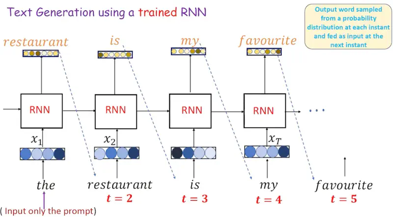
- Text Generation (One to Many)
- Sentiment Classification (Many to One)
- Machine Translation (Many to Many)
Note: The input \(x_1, x_2, \dots, x_T \) are the vector representations of the words or word embeddings, earlier OHE was used, but after 2013, Word2Vec or GloVe etc. are mostly used.
Text Generation (One to Many)
We just give one word as input to the RNN, and it keeps on generating text, by just keep predicting the next word.
Therefore, one-to-many mapping.
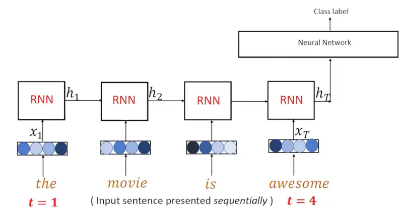
Sentiment Classification (Many to One)
We give a sentence as input for which we want the RNN to predict the sentiment as positive, negative or neutral, and we just get that one word as output.
For sentiment analysis, the RNN take the sentence as input and generates an encoded hidden state \(h_T\) for the entire sentence as output.
And this encoded vector representation of the sentence \(h_T\) is fed into another simple neural network for classification of the sentiment.
Hence, it is of the kind many-to-one mapping.
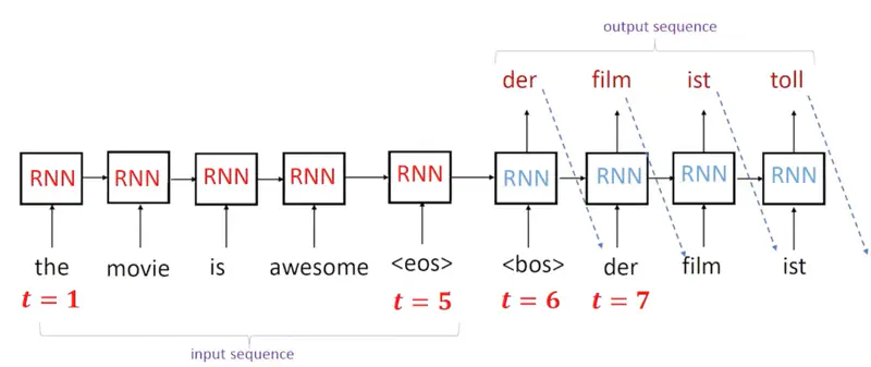
Machine Translation (Many to Many)
Machine Translation means language translation, here we use 2 RNNs, one as encoder for encoding the input language sentence,
and another RNN as decoder for generating the translated language sentence.
Hence, many-to-many mapping.
Encoder Decoder Architecture
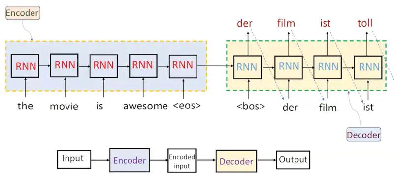
Note: The Red(encoder) and Blue(decoder) RNN blocks are different with different parameters.
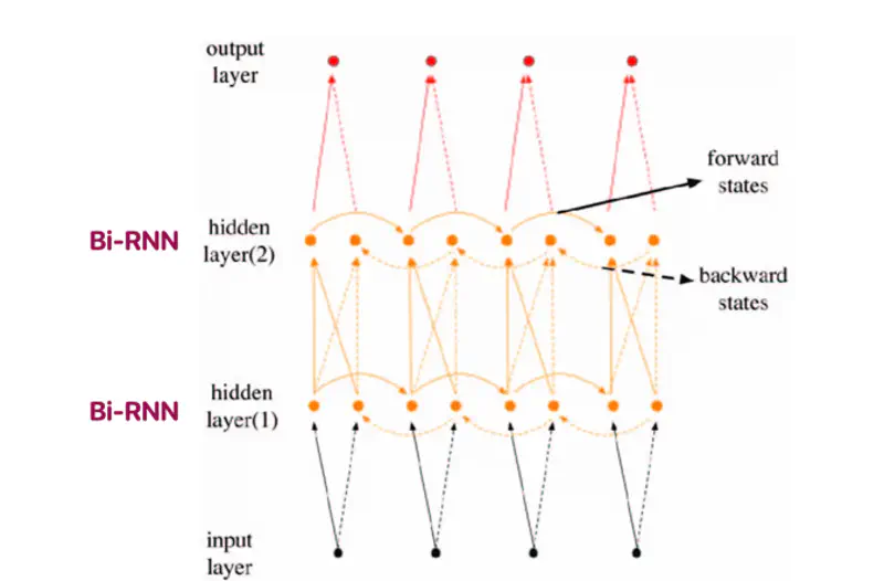
- Bi-Directional RNN (Bi-RNN)
- Multi-Layer Bi-RNN
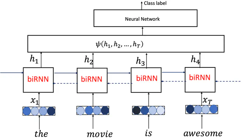
Bi-RNN
Processes sentences by analyzing it in both forward and backward directions.
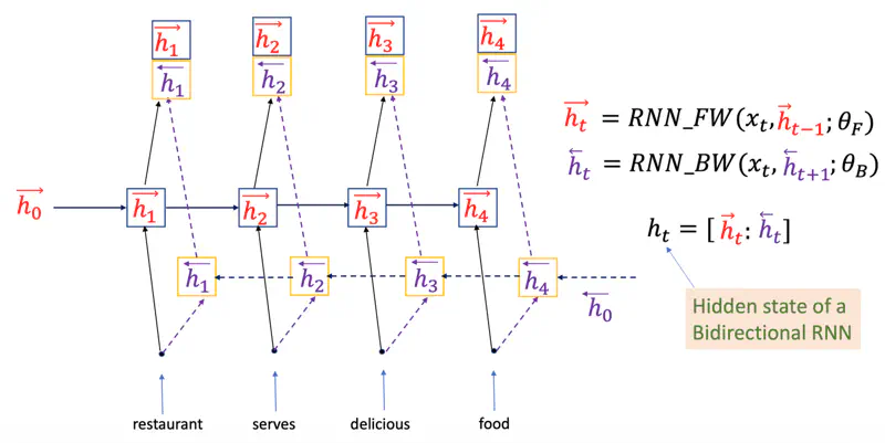
We can use Bi-RNN for sentence classification, and it will perform better than vanilla RNN, because it processes the sentence from both forward and backward direction, hence it has better and more rich context.
Sentence Classification
Multi Layer Bi-RNN
Stacking multiple Bi-RNN layers allows the model to learn complex patterns and high-level representations.