Self Attention
4 minute read
RNNs process words sequentially, i.e, one by one.
- To understand word 20, you must first process words 1 to 19.
- By the time the model gets to the end of a long sentence, it often “forgets” the beginning (vanishing gradient problem).
Read more about Vanishing Gradient Problem
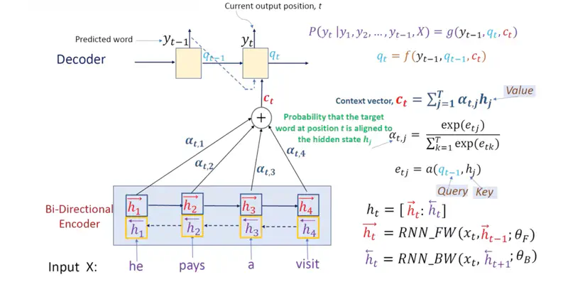
Note: Luong Attention (2015) used “dot product” based attention was faster than Bahdanau Attention (2014) (additive), but was still RNN based Seq2Seq model.
In 2017, Transformer architecture, proposed that “Self-Attention” can be used completely for machine translation instead of RNNs.
Using “Self-Attention” made the model highly parallelizable because the matrix calculations can be done on GPUs in parallel.
Transformer Architecture
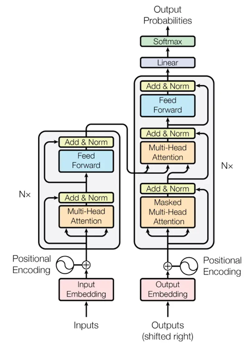
Research Paper: Attention Is All You Need, Vaswani et al. , 2017, https://arxiv.org/pdf/1706.03762
Primary reason we need self-attention is that words do not have a fixed meaning; their meaning is defined by their neighbors and context.
Example
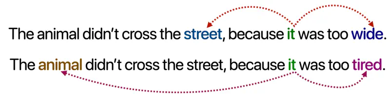
Note: Depending upon the context “it” will refer to “street” or “animal”.
Unlike older models that read left-to-right, self-attention sees the whole sentence at once, allowing it to catch relationships whether they are side-by-side or miles apart.
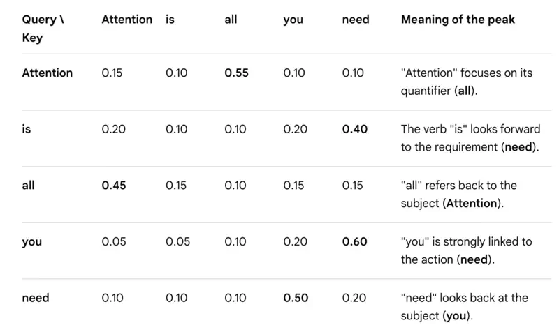
Every word in a sentence looks at every other word (including itself) to decide which word is most relevant to its own meaning in that specific context.
Self-Attention
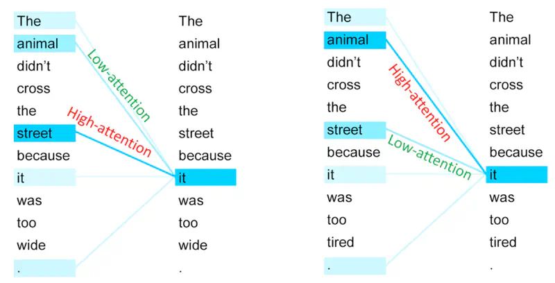
In the first sentence, “it” pays ‘high attention’ to street and ’low attention’ to animal.
And, in the second sentences, “it” pays ‘high attention’ to animal and ’low attention’ to street.
Unlike RNNs, the calculation for a token does not depend on the computation of the previous token.
All tokens can attend to all other tokens at the same time, i.e,
the attention scores (dot products between ‘\(q\)’ and ‘\(k\)’) are computed for all pairs of tokens simultaneously on GPU cores, not one-by-one.
Attention Mechanism
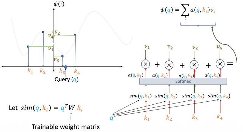
The attention score (\(q,k,v\)) for a query ‘\(q\)’, given keys ‘\(k_i\)’ and values ‘\(v_i\)’ is the summation of all query and key similarity scores similarity(\(q, k_i\)) multiplied by their corresponding values ‘\(v_i\)’.
- Query (\(q_i = W_Q^T x_i\)): “What am I looking for?”
- Key (\(k_i = W_K^T x_i\)): “What do I offer?” (The label others use to find me).
- Value (\(v_i =W_V^T x_i\)): “What information do I actually carry?”
Note: \(x_i \in \mathbb{R}^{d_{model} \times 1}\)is the input word vector and \(W^Q, W^K \in \mathbb{R}^{d_{model} \times d_k} \text{ and } W^V \in \mathbb{R}^{d_{model} \times d_v}\)are learned weight matrices.
Individual Attention
The “match” between two words is calculated using a “dot product”.
If word ‘\(i\)’ wants to know how much it should care about
word ‘\(j\)’, it compares its ‘Query’ to the other word’s ‘Key’:
Self Attention Score
We pack all the individual queries, keys, and values into matrices \(Q, K, \text{ and } V\), where,
Note: ‘\(k\)’ is the dimension of \(Q, K, V\) vectors.
Self Attention Example
Why do we scale the dot product ?
\[\text{Attention}(Q, K, V) = \text{softmax}\left(\frac{QK^T}{\sqrt{d_k}}\right)V\]Research paper says that -
“We suspect that for large values of \(d_k\), the dot products grow large in magnitude,
pushing the softmax function into regions where it has extremely small gradients.
To counteract this effect, we scale the dot products by \(\frac{1}{\sqrt{d_k}}\)”
Gradient of Softmax:
\[\frac{\partial \sigma_i}{\partial z_j} = \begin{cases} \sigma_i(1 - \sigma_i) & \text{if } i = j \\ -\sigma_i\sigma_j & \text{if } i \neq j \end{cases} \]Combining both cases:
\[\frac{\partial \sigma_i}{\partial z_j} = \sigma_i (\delta_{ij} - \sigma_j)\]where, \(\delta_{ij}\) is the Kronecker delta (1 if \(i=j\) (diagonal), 0 otherwise).
e.g., say, if Softmax (\(\sigma_i\)) = 0.99,
then gradient \(\frac{\partial \sigma_i}{\partial z_j} = \sigma_i(1 - \sigma_i) = (0.99)*(0.01) = 0.0099 \)
which is a very low value, so the weight updates will effectively be negligible.
Dividing by \(\sqrt{d_k}\) reduces the variance back to 1, keeping the scores in a moderate range.
Therefore, the scaling factor \(\frac{1}{\sqrt{d_k}}\) acts as a stabilizer, preventing the model from having extreme confidence in a few places, which enables smoother training.