Text Representation

Text Representation - OHE, BoW, TF-IDF, Word2Vec, GloVe, FastText

10 minute read

PlaylistNatural Language Processing | Full Course

Text Representation

Process of converting raw text into numerical vectors that machines can understand.

We will discuss the following ways to represent text as vectors:

One Hot Encoding (OHE) (discrete)
Bag of Words (BoW), TF-IDF (statistical)
Word2Vec, GloVe, FastText (distributed)

Requirements of Good Text Representation

Capture meaning/similarity (semantics)
Capture context
Compact

One Hot Encoding

Every word in the vocabulary ‘V’ is assigned a unique index.

e.g.

\[ \mathbf{v_{aardvark}} = \begin{pmatrix} 1 \\ 0 \\ 0 \\ \vdots \\ 0 \end{pmatrix}, \mathbf{v_{abacus}} = \begin{pmatrix} 0 \\ 1 \\ 0 \\ \vdots \\ 0 \end{pmatrix}, \dots , \mathbf{v_{zyzzyva}} = \begin{pmatrix} 0 \\ 0 \\ 0 \\ \vdots \\ 1 \end{pmatrix} \]

Limitations

High dimensional (curse of dimensionality)
Sparse vectors
No semantics is captured
- e.g., “love” vs “like” → completely different vectors

Bag of Words

Represents a document by the frequency of words within it, disregarding grammar and word order.

Given a sequence of words in a document, \(D: <(w_1, w_2, \dots , w_T>\).
Vocabulary, \(\mathbf{v}_D = \sum_{i=1}^T \mathbf{v}_{w_i}\)

e.g. Document, D = “We learn NLP. For NLP we need to learn BoW."

Vocabulary = [“We”, “Learn”, “NLP”, “For”, “Need”, “To”, “BOW”]
Vector = [ 2, 2, 2, 1, 1, 1, 1]

Limitations

Stop Word Problem: Common words like “the” or “is” appear frequently but carry little information, often drowning out the meaningful terms.
Sparse Vector.
Semantics not captured.
Word ordering is not captured.
- e.g. \( \mathbf{v_{\text{man kills lion}}} = \begin{pmatrix} 0 \\ \vdots \\ 1 \\ 0 \\ \vdots \\ 1 \\ 0 \\ \vdots \\ 0 \\ 1 \\ \vdots \\ \end{pmatrix} = \mathbf{v_{\text{lion kills man}}} \)

Term Frequency-Inverse Document Frequency (TF-IDF)

To solve the stop-word problem, TF-IDF penalizes words that appear across almost all documents.

Term Frequency (TF): Measures how frequently a term ‘t’ occurs in a document ‘d’.
- \(TF(t, d) = \frac{\text{Number of times } t \text{ appears in } d}{\text{Total number of words in } d}\)
Inverse Document Frequency (IDF): Measures how important a term is across the entire corpus ‘D’.
- \(IDF(t, D) = \log\left(\frac{\text{Total number of documents } N}{\text{Number of documents containing term } t}\right)\)
\(TF-IDF(t, d, D) = TF(t, d) \times IDF (t, D)\)

If a word appears in every document (like “the,” “is,” “data”), it isn’t a good discriminator.

Note: The log function “dampens” the effect of very high frequencies.

TF-IDF Score Meaning

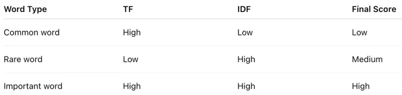
images/natural_language_processing/text_representation/tfidf_meaning.png

The minimum TF-IDF value is 0. This occurs when a term appears in all documents (IDF = 0) or is not present in the document at all (TF = 0).
No fixed upper bound for unnormalized TF-IDF; Max value depends on the corpus size (\(log(\text{Number of Documents})\)) and how rarely a word appears.

Let’s understand the TF-IDF score better with a very simple example.

Document 1: “I love coffee.”
Document 2: “I love tea.”
Vocabulary: {‘I’, ’love’, ‘coffee’, ’tea’}
Output Matrix:

	I	Love	Coffee	Tea
Doc 1	0	0	0.1	0
Doc 2	0	0	0	0.1

Limitations

Semantics not captured, e.g car ≠ vehicle.
Word ordering is not captured.
Sparse Vector.
- Vector size = vocabulary size;
- For a vocabulary of 50,000 words, every document is a 50,000-dimensional vector consisting mostly of zeros.
No context awareness, e.g., “bank” (river) vs “bank” (finance).
Corpus dependency.
- Changing corpus changes representation.
Poor generalization.
- New/unseen words → no representation

Note: TF-IDF answers → “Which words are important in this document?” , but NOT “What does this word mean?”.

Distributed Text Representation

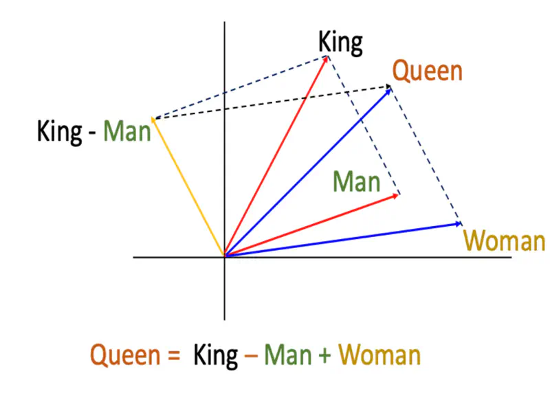
Till now, we have seen that complete semantic information of each word is mapped to exactly one dimension in the vector, such as, OHE, BoW, and TFIDF.

Wouldn’t it be better if we captured the semantic and syntactic information separately in different dimensions such that similar words have similar vectors and the representation generalizes well.

e.g. Say, a word like “Apple” is represented by a 300-dimensional vector.

Dimension 1 might represent “fruitiness,”
Dimension 2 “redness,” and
Dimension 3 “technology.”
and so on …

💡 If we are able to represent a word in multiple dimensions then we can compare words in those multiple dimensions on various aspects, such that all the similar words occur together.

Distributed Representation of Words

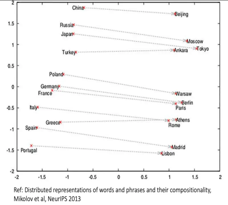
images/natural_language_processing/text_representation/distributed_representation_1.png

images/natural_language_processing/text_representation/distributed_representation_2.png

Note: We can see that similar words occur together.

Video Word Embeddings (Vector) | OHE | Bag of Words | Term Frequency Inverse Document Frequency (TFIDF)

Word2Vec

“You shall know a word by the company it keeps.” ~ J.R. Firth, 1957

Word2Vec captures information about the meaning of the word based on the surrounding words, because meaning comes from context.

Developed at Google (Mikolov et al.), 2013.
Word2Vec moved NLP from “counting” to “predicting”.

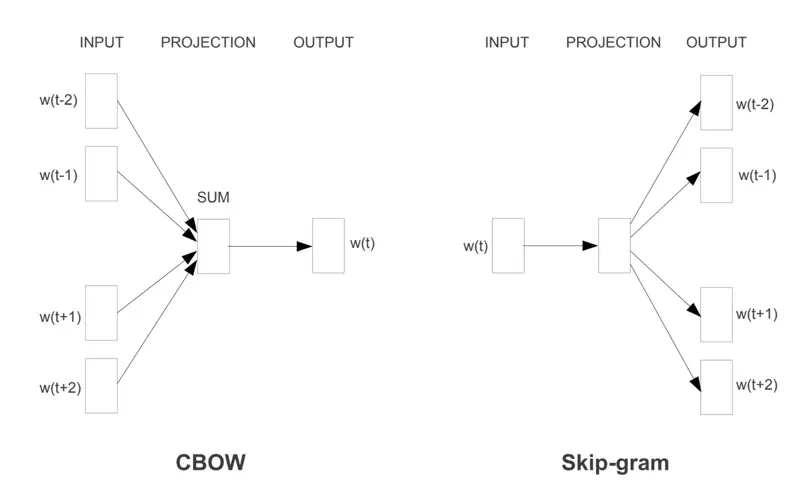
Word2Vec uses 2 methods to learn one vector per word appearing in the corpus.

CBOW (Continuous Bag of Words): Predicts a target word based on its context (the surrounding words).
- Best for: Smaller datasets; smooths over some noise.
Skip-gram: Predicts the context words given a single target word.
- Best for: Large datasets; better at representing rare words.

Word2Vec Architectures

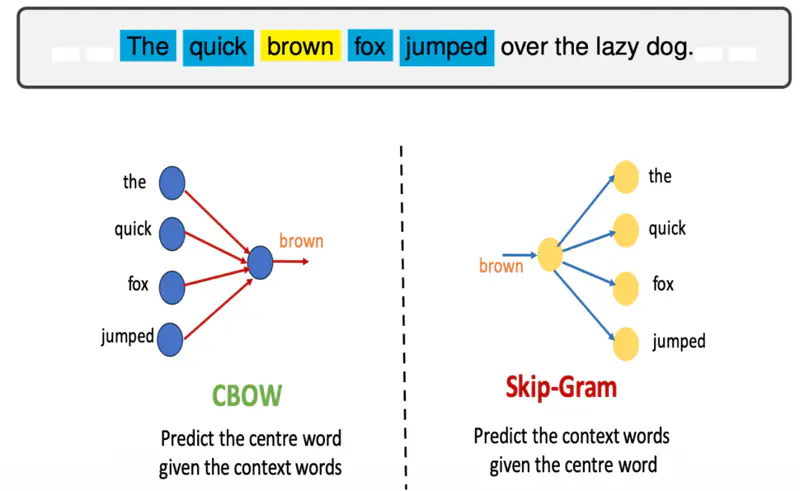
images/natural_language_processing/text_representation/word2vec_example.png

Skip-Gram

Skip-Gram predicts the surrounding context words given the center or target word.
It operates on the principle that words appearing in similar contexts tend to have similar semantic meanings, making it effective at capturing both semantic and syntactic relationships.

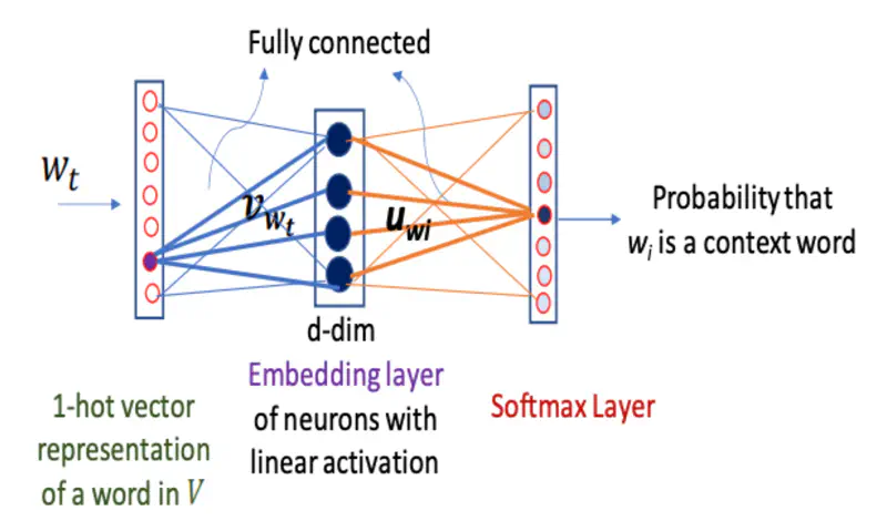
images/natural_language_processing/text_representation/skip_gram_2.png

\[P(\mathbf{w}_i \text{ is a context word} | \mathbf{w}_t) = \frac{exp(\mathbf{v}^T_{w_t}\mathbf{u}_{w_i})}{\sum_{w \in V} exp(\mathbf{v}^T_{w_t}\mathbf{u}_{w})}\]

If the training example is “brown”, then the softmax output corresponding to the word “fox” will be 1, rest all units will be 0.

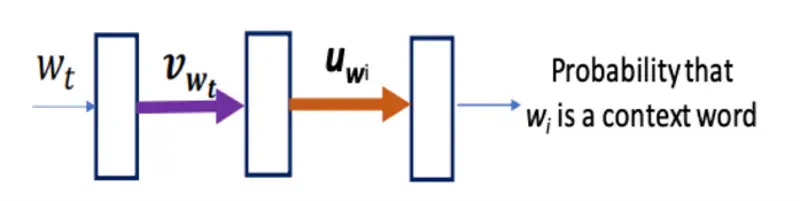
Note: \(\mathbf{v}_{w_t}\) is used as the final dense vector representation for the word \(w_t\).

Negative Sampling

Let’s dive deeper into Skip-Gram architecture and understand the optimization problem.
Cost Function

\[log ~ P(w_{t+j} | w_t) = \mathbf{v}^T_{w_t}\mathbf{u}_{w_{t+j}} - log\sum_{w \in V} \mathbf{v}^T_{w_t}\mathbf{u}_{w}, \quad j = −k, . . . , k; j \ne 0\]

Problem
Here, the computation of probability of context word given center word \(P(w_{t+j} | w_t)\), and its derivative, i.e, \(\frac{\partial {P(w_{t+j} | w_t)}}{\partial {\mathbf{v}_{w_t}}}\) (for gradient descent weight update) is expensive if vocabulary size is large, i.e, \(|V| \gg 0\).

Note: Loss Function = Cross Entropy

Computational Scale Analysis
If our vocabulary has \(10^{5}\) words, every single update for a single word pair requires \(10^{5}\) operations.
Since a typical corpus has billions of tokens, performing \(|V|\) operations per token makes training mathematically possible but computationally intractable on standard hardware.

Solution
Negative Sampling
A clever trick !
Instead of summing over the whole vocabulary, the model only updates the “true” context word and a small sample (e.g., 5–20) of random “negative” words.
This turns a massive multiclass classification problem into a series of simple binary logistic regression problems.

Randomly select a small number of ‘K’ non-context words for which softmax unit output is 0.
For every “Positive” pair (words that actually appear together), we generate ‘K’ “negative” pairs (words that are randomly sampled from the dictionary and likely have no relationship).
- Positive Pair (\(w, c\)): “The quick brown fox” \(\rightarrow\)(quick, fox)
- Negative Pairs (\(w, c_{neg}\)): (quick, apple), (quick, potato), (quick, diary)

Benefit: If we have a vocabulary of 10,000 words and use , we only update weights for 6 output neurons (1 positive + 5 negative) instead of all 10,000.

How Negative Sampling Works ?
Cost Function

\[log ~ \hat{P}(w_{t+j} | w_t) = \underbrace{log(\sigma(\mathbf{v}^T_{w_t}\mathbf{u}_{w_{t+j}}))}_{Positive Pair} + \sum_{k=1}^K \underbrace{log(\sigma(-\mathbf{v}^T_{w_t}\mathbf{u}_{w}))}_{Negative Pair}\]

🎯 Goal is to maximize the log likelihood function.

We can see that both the terms on the left of equality is of the form \(log(\sigma(x))\), where \(x\) is the dot product \(v^Tu\).
Since, sigmoid function outputs value in the range of 0 to 1, so \(log(\sigma(x))\) range will be \((-\infty, 0]\).
Therefore, in order to maximize the value of log likelihood we need to bring it closer to 0.

Let’s see how the values of \( x, \sigma(x)\), and \(log(\sigma(x))\) vary together:

Positive Pair: as \(x \rightarrow \infty, ~ \sigma(x) \rightarrow 1, ~ and ~ log(x) \rightarrow 0\)
Negative Pair: as \(x \rightarrow -\infty, ~ \sigma(x) \rightarrow 0, ~ and ~ log(x) \rightarrow -\infty\)

Note: \(\sigma(-x) = 1 - \sigma(x)\)

Video Word2Vec Embedding | Detailed Explanation with Maths | Skip Gram | CBOW | Negative Sampling

Global Vectors (GloVe)

Limitation of Word2Vec
Word2Vec only uses local context and is excellent at analogies and capturing semantics but ignores the vast amount of statistical information available in the global co-occurrence counts.
As, we saw earlier in the case of TF-IDF that uses the statistics of the entire corpus.

GloVe leverages global co-occurrence matrix, allowing it to better understand how words relate across the entire dataset, resulting in superior semantic analogies and better representation of relationships between distant words.

Research Paper: GloVe: Global Vectors for Word Representations, Pennington et al., Stanford University, 2014, https://nlp.stanford.edu/pubs/glove.pdf

Glove model leverages statistical information by training only on the nonzero elements in a word-word co-occurrence matrix, and uses matrix factorization to generate low-dimensional word representations.

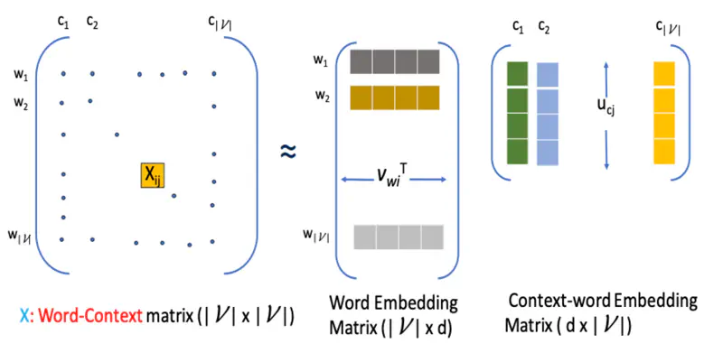
images/natural_language_processing/text_representation/glove.png

\(X_{ij}\) : Number of times word \(c_j\) appears in the context of word \(w_i\)

Word-word matrix or word-context matrix \(X\) is factorized into 2 matrices, such that:

\[X_{ij} \approxeq \mathbf{v}^T_{w_i}\mathbf{u}_{c_j} \text{ or } X_{ij} \approxeq exp(\mathbf{v}^T_{w_i}\mathbf{u}_{c_j})\]

Note: We do an exponentiation because dot product can be negative but the word count is always positive.

We have to find the 2 matrices such that the difference between the dot product and the actual word co-occurrence count is minimum.
This can be formulated as an optimization problem, because we have to find some kind of optimum, in this case minimum value.

Optimization Problem

\[ \underset{\mathbf{v}_w, \mathbf{u}_c}{\mathrm{min}} \lVert \mathbf{V}_w \mathbf{U}_c - \text{log}(\mathbf{X}) \rVert^2_F \]

where, F is Frobenius Norm

Estimate word and context vectors by solving the optimization problem:

\[ \underset{\mathbf{v}_w, \mathbf{u}_c, b, \tilde{b}}{\mathrm{min}} \sum_{i,j=1}^{|V|} f(X_{ij}) ~ ( \mathbf{v}^T_{w_i}\mathbf{u}_{c_j} + b_i + \tilde{b}_j - \text{log}(X_{ij}))^2\]

\[f(x) = \begin{cases} (x/x_{max})^{\alpha} & \text{if } x < x_{max} \\ 1 & otherwise \end{cases} \]

Note: In the paper they empirically found that the most suitable value of \(\alpha = 3/4\).

Let’s understand all the parameters.

\(f(X_{ij})\): Weighting function.
- If \(X_{ij} = 0\): \(f(x) = 0\); Ignore pairs that never co-occur.
- If \(X_{ij}\) is small: \(f(x)\) is also small, but increases as count increases.
- If \(X_{ij}\) is very large (for stop words): \(f(x)\) saturates (usually at 1); prevents common stop-words from over-influencing the vectors.
Bias terms
- \(b_i\): Captures the “inherent frequency” of the target word \(w_i\).
  - If word \(w_i\) is very common (like “the”), \(b_i\) will be large.
- \(\tilde{b}_j\): Captures the “inherent frequency” of the context word \(c_j\).

Comparison: GloVe Vs Word2Vec

✅ GloVe can often outperform Word2Vec on smaller datasets because it extracts more statistical signal from every available word pair.
✅ Pre-trained Word2Vec models are often significantly larger (e.g., 3.4GB for Google News) compared to GloVe’s more lightweight variants (e.g., 150MB for Wiki-Gigaword), making GloVe better for resource-constrained applications.
✅ In practice, we start with GloVe for its stability and availability of pre-trained vectors, then experiment with Word2Vec if the specific syntactic nuances of their dataset are not being captured.

Video Global Vectors (GloVe) Embedding | Detailed Explanation | Matrix Factorization | Word2Vec Vs GloVe

FastText

Instead of treating each word as an atomic unit, FastText breaks words into a “bag” of character ’n-grams’ (skip-gram), which allows it to capture morphological information and effectively handle rare or out-of-vocabulary (OOV) words.

Developed by Facebook AI Research (FAIR).

e.g. if n = 3, (typically, n = 3, 4, 5, 6):
<where> : { <wh, whe, her, ere, re>, <where>}

Note: FastText also uses Skip-Gram architecture, similar to Word2Vec, wo we will not discuss skip gram model and dive in directly into understanding the difference between FastText and Word2Vec approaches.