Transformer
6 minute read
Transformer replaced recurrence with attention, enabling faster training and superior performance in NLP and AI tasks.
Source: Attention is all you need, Vaswani et al., 2017; https://arxiv.org/pdf/1706.03762
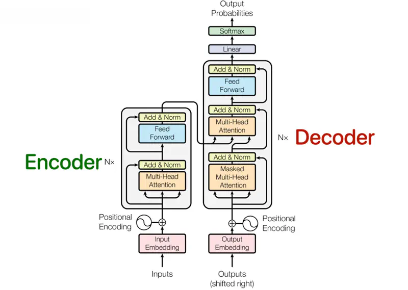
Transformer Architecture
It was designed for machine translation, so it has 2 parts, viz., encoder and decoder.
Encoder
The encoder is composed of a stack of N = 6 identical layers.
- Each encoder layer has 2 sub-layers:
- Multi-Head Self Attention
- Fully connected Neural Network (Feed Forward)
- Residual connection around each of the sub-layers.
- Each sub-layer has layer normalization.
Decoder
The decoder is also composed of a stack of N = 6 identical layers.
- Each decoder layer has 3 sub-layers:
- Masked Multi-Head Attention
- Multi-Head Encoder Decoder (Cross) Attention
- Fully connected Neural Network (Feed Forward)
- Residual connection around each of the sub-layers.
- Each sub-layer has layer normalization.
Transformer replaced recurrence with attention.
3 kinds of attention are used in the transformer architecture:
- Multi-Head Self Attention (Encoder)
- Masked Multi-Head Attention (Decoder)
- Encoder Decoder (Cross) Attention (Decoder)
Unlike older models that read left-to-right, self-attention sees the whole sentence at once, allowing it to catch relationships whether they are side-by-side or miles apart.
Every word in a sentence looks at every other word (including itself) to decide which word is most relevant to its own meaning in that specific context.
We have discussed self attention in detail in the previous article.
In a single-head attention system, the model has to condense all relationships into one attention score.
e.g., The Reserve Bank of India headquarters in Mumbai, sits on the bank of the Mithi River.
If a word like “bank” refers to both a “river” and “financial institution” in a complex sentence,
a single head tries to average those two different meanings.
By averaging them, we often end up with a blurry representation that does not capture either meaning well.
Allows the model to “dissect” the word.
Each head can look at different aspects of a sentence, such as, syntax (subject-verb), semantics(meaning), pronouns, etc.
- Head 1 can focus on the “river” context while
- Head 2 focuses on the “financial institution” context.
- No need to compromise (average).
- Also, each head can be processed in parallel.
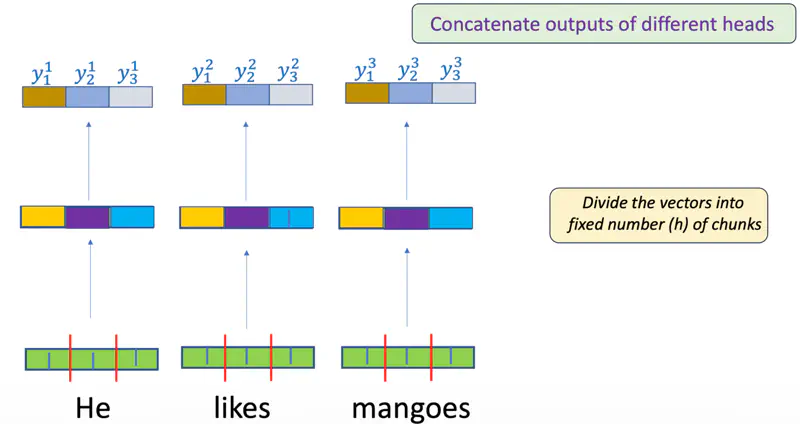
Multi-Head Attention
Multi-Head
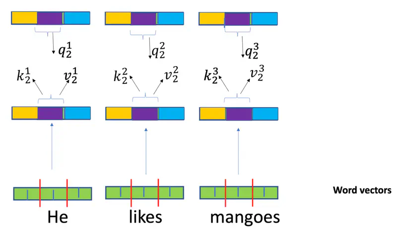
Each head is an independent attention mechanism.
Each head has its own set of learnable weight matrices (\(W_i^Q, W_i^K, W_i^V\)).
In decoder (auto-regressive), a token can only see itself and the tokens that came before it.
So, we add a mask to hide the future words.
where,\(M\): Mask (a square matrix of the same size as the attention scores).
- \(M = 0\): for positions we want to keep (“past” and “current” tokens)
- \(M = 1\): for positions we want to hide (“future” tokens).
e.g.
\[M = \begin{bmatrix} 0 & -\infty & -\infty \\ 0 & 0 & -\infty \\ 0 & 0 & 0 \end{bmatrix}\]Note: Softmax function is what actually performs the “masking” by turning those ‘\(-\infty\)’ values into zeros.
The “queries” come from the previous decoder layer, and the “keys” and “values” come from the output of the encoder.
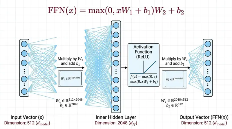
Fully connected Feed Forward Network introduces non-linear activation functions that allows the model to learn complex, non-linear relationships that attention(linear operation) alone cannot capture.
\[FFN(x) = max(0, xW_1 + b_1)W_2 + b_2 \]Feed Forward Network
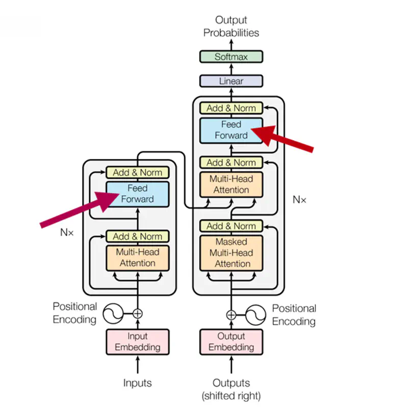
Note: The dimensionality of input and output is \(d_{model}\) = 512, and the inner-layer has dimensionality \(d_{ff}\) = 2048.
- Residual connection is used to mitigate the vanishing gradient problem.
- Skip-connections allow original input features to skip layers and be preserved, which helps the model avoid losing information in deep networks.
- But, the most vital role of residual connection is to solve the “degradation problem”.
Degradation Problem
Counter-intuitively, as model depth increases, accuracy tends to saturate and then degrade rapidly;
not because of overfitting, but because of optimization failure.
In a deep neural network (without residuals), the optimization surface becomes so rugged and chaotic that
it becomes very difficult to reach the local minima through gradient descent.
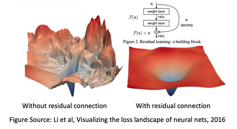
Note: A layer can simply pass the input through unchanged (identity mapping) if it does not find useful features.
Unlike Batch Normalization, which normalizes across the mini-batch for each individual feature, Layer Normalization normalizes across all the features (dimensions) for a single training instance.
- By centering mean (\(\mu\)) around zero and scaling them to variance (\(\sigma^2\)) of one, it prevents exploding or vanishing gradients, enables faster convergence.
- The mean (\(\mu\)) and variance (\(\sigma^2\)) are calculated over all features(dimensions) for that specific token.
Reason: Transformers primarily use LayerNorm because it treats each token independently.
This is critical for natural language processing (NLP) where sentences in a batch often have different lengths.
Limitations of Self Attention
Self-attention mechanism treats a sentence as a set of tokens rather than a sequence, it is inherently permutation-invariant.
e.g. “Cat eats fish.” is same as “Fish eats cat.”
Positional Encoding
So, in order to differentiate the relative position of words, Transformer architecture introduced positional encoding.
where, ‘\(pos\)’: position and ‘\(i\)’: dimension
In simple, terms each position ‘\(pos\)’ is encoded using sine and cosine functions.
This was mainly chosen to easily represent the ‘relative position’ of two words as a linear function.
Note: The formula uses \(i\) (the dimension index) to vary the frequency of the sine/cosine waves across the \(d_{model}\)-dimensional vector.
Relative Position
Say, we want to know the relative position for a word that is ‘\(k\)’ steps away.
- Position of word 1: ‘\(pos\)’ 
- Position of word 2: ‘\(pos\)’+ ‘\(k\)’
We know that:
\[\sin(A + B) = \sin(A)\cos(B) + \cos(A)\sin(B)\]\[\cos(A + B) = \cos(A)\cos(B) - \sin(A)\sin(B)\]\[\sin(pos + k) = \sin(pos)\cos(k) + \cos(pos)\sin(k)\]\[\cos(pos + k) = \cos(pos)\cos(k) - \sin(pos)\sin(k)\]So, we can represent the relative position of the second word at ‘\(pos\)’+ ‘\(k\)’, as a linear function of first word at ‘\(pos\)’.
\[\begin{bmatrix} \sin(pos + k) \\ \cos(pos + k) \end{bmatrix} = \begin{bmatrix} \cos( k) & \sin(k) \\ -\sin(k) & \cos(k) \end{bmatrix} \begin{bmatrix} \sin(pos) \\ \cos(pos) \end{bmatrix}\]All the information about Transformer architecture ends here, and the below positional encoding techniques are not a part of transformer architecture.
Just adding them here for the time being, because the concepts are related.
RoPE positional encoding is used in Llama and Mistral LLMs.
Does not add a vector to the embedding, instead, it rotates the Query (\(Q\)) and Key (\(K\)) vectors in 2D planes.
After rotation, when we take the dot product, we automatically get the relative position of tokens.
where ‘\(m\)’ is the position
Ignores the embeddings entirely and modifies the attention scores directly.
For every head, we subtract a penalty from the attention score proportional to the distance between tokens.
where ‘\(m\)’ is a head-specific slope